CS 180 Project 1: Images of the Russian Empire

Ryan Campbell

Introduction

Between 1909 and 1915, Sergey Mikhaylovich Prokudin-Gorsky travelled across the Russian Empire and documented a variety of things through photography. Interestingly, despite this being well before the time of widespread color photography, his records give us a colorful insight into the Russian Empire. This is because he was ingenious enough to capture three exposures of every photo, using a red, green, and blue filter.

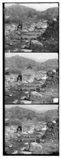
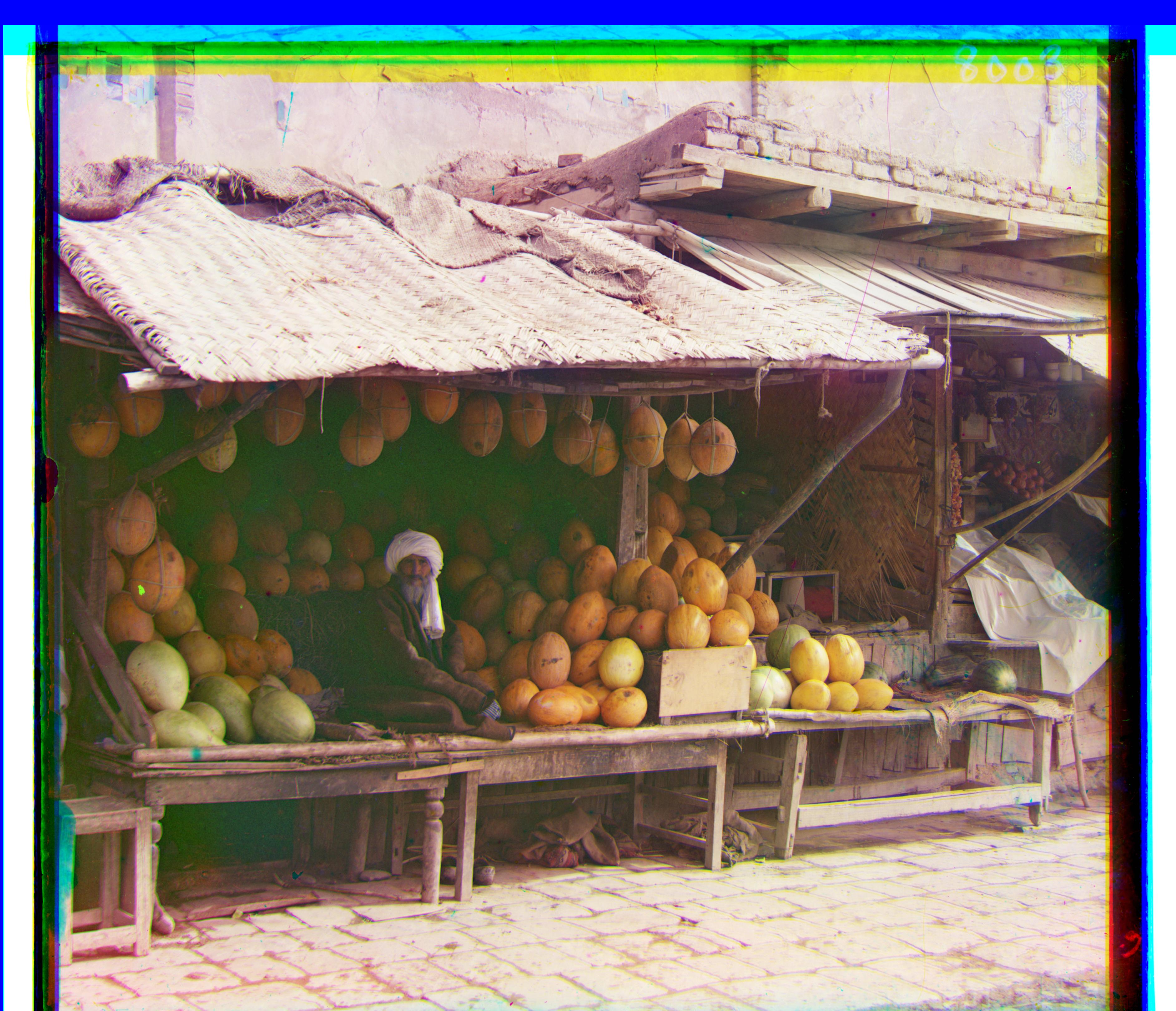
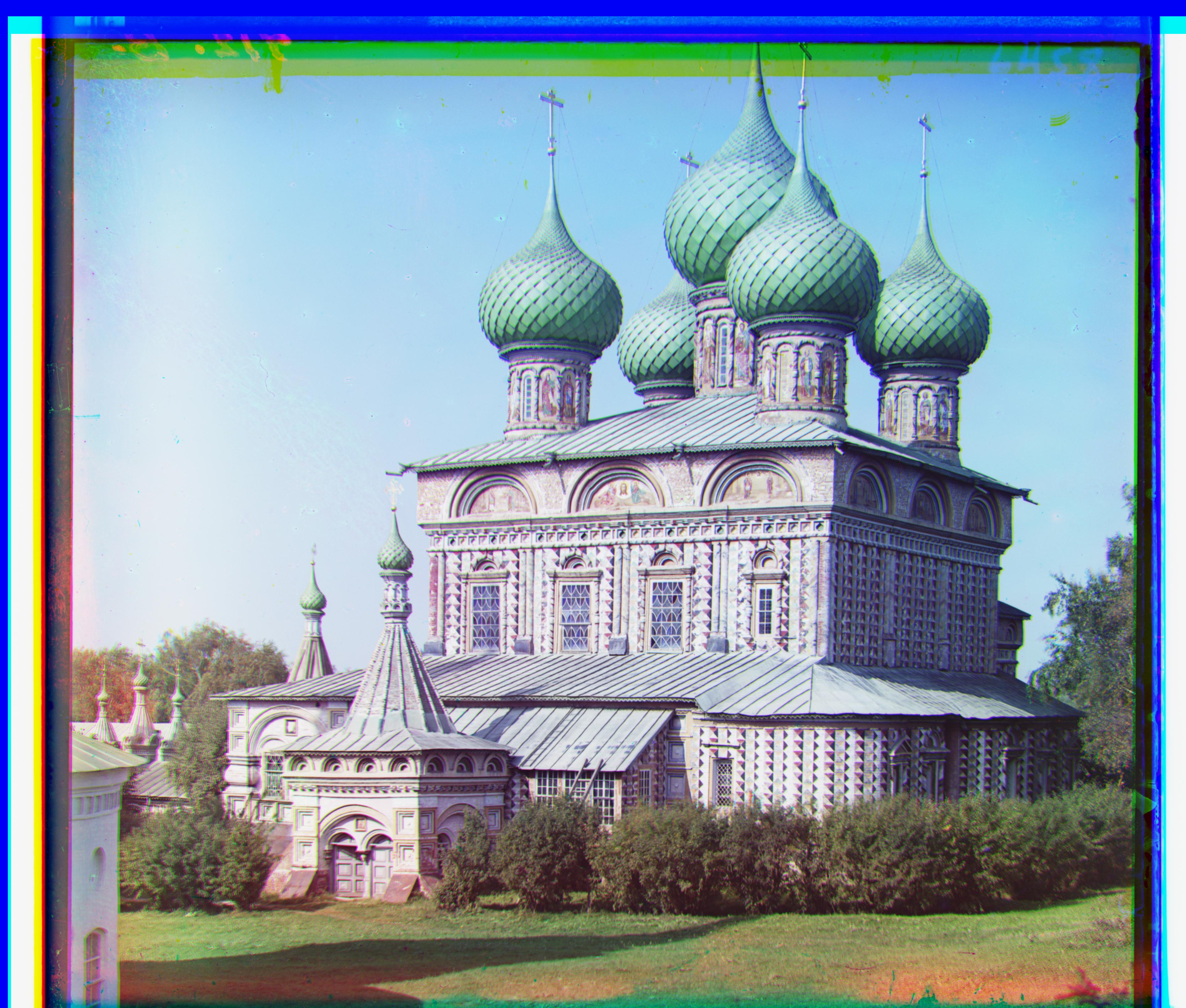
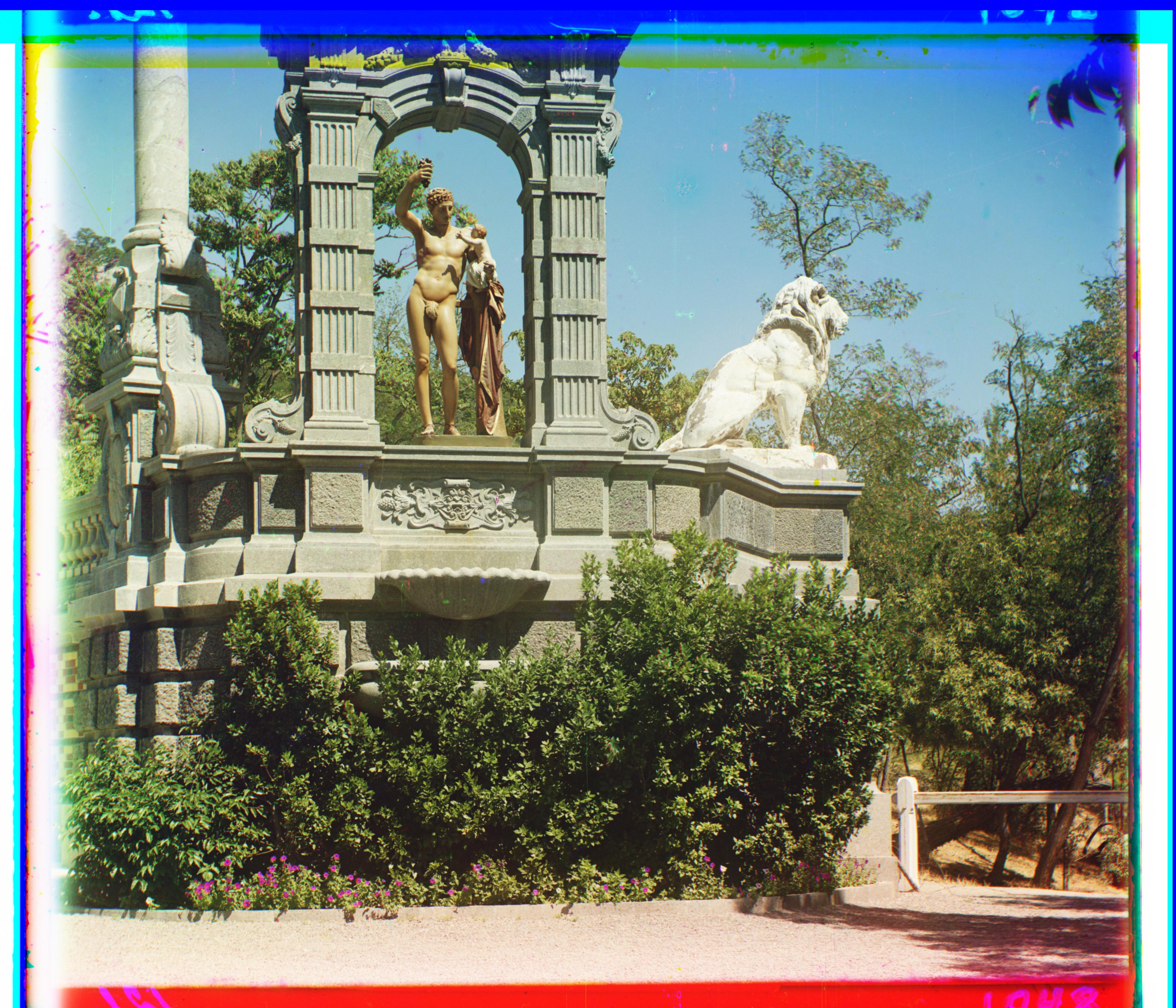
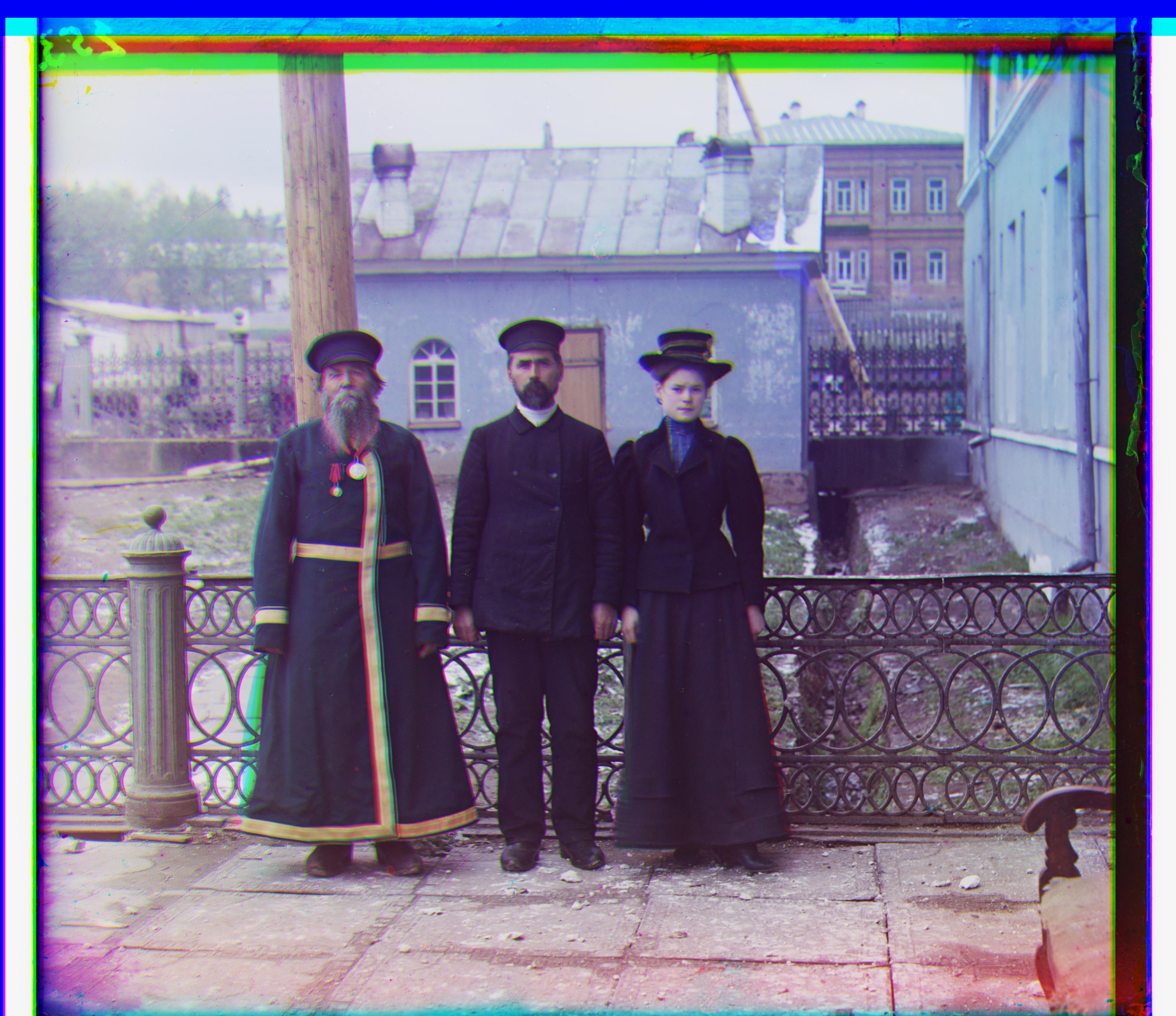
Now, his photographs have been digitized by the Library of Congress. Each image is a vertical stack of the individual images captured by the blue, green, and red filters.

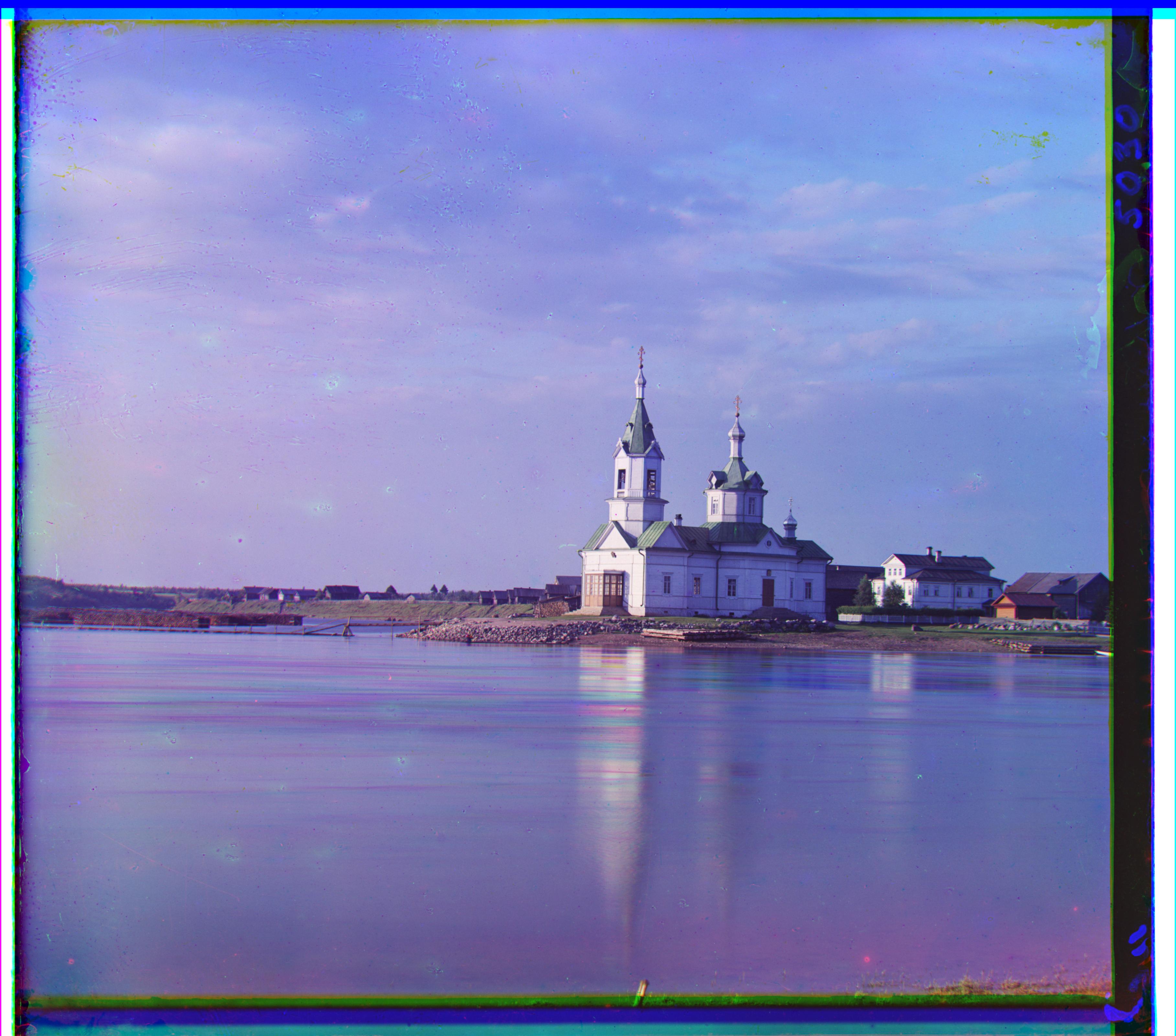
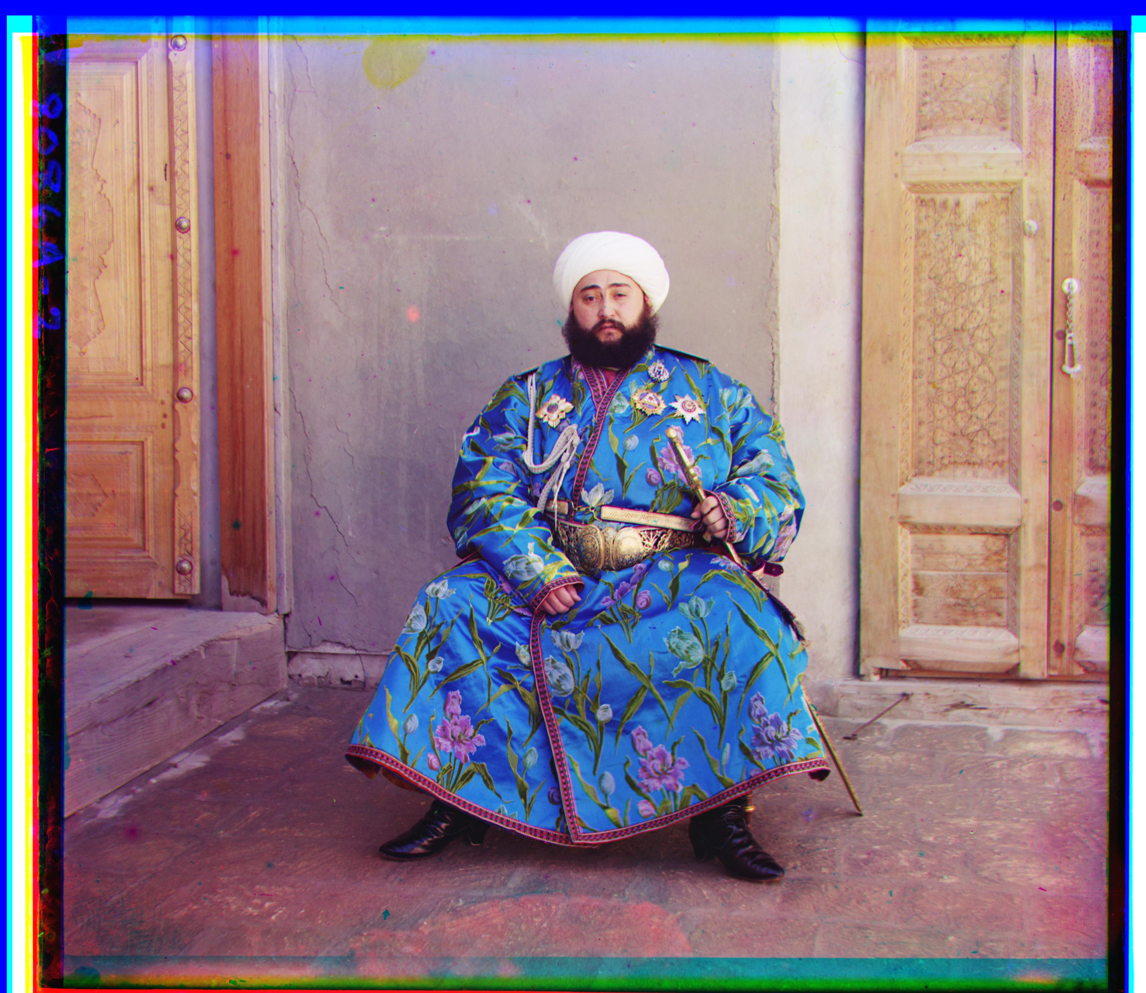
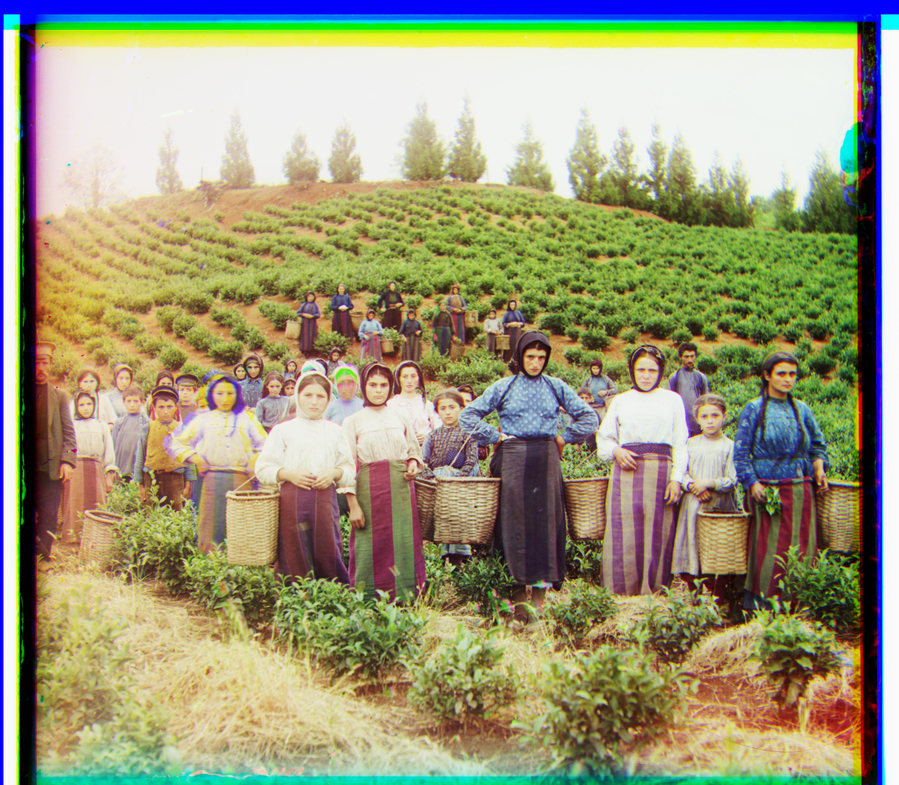
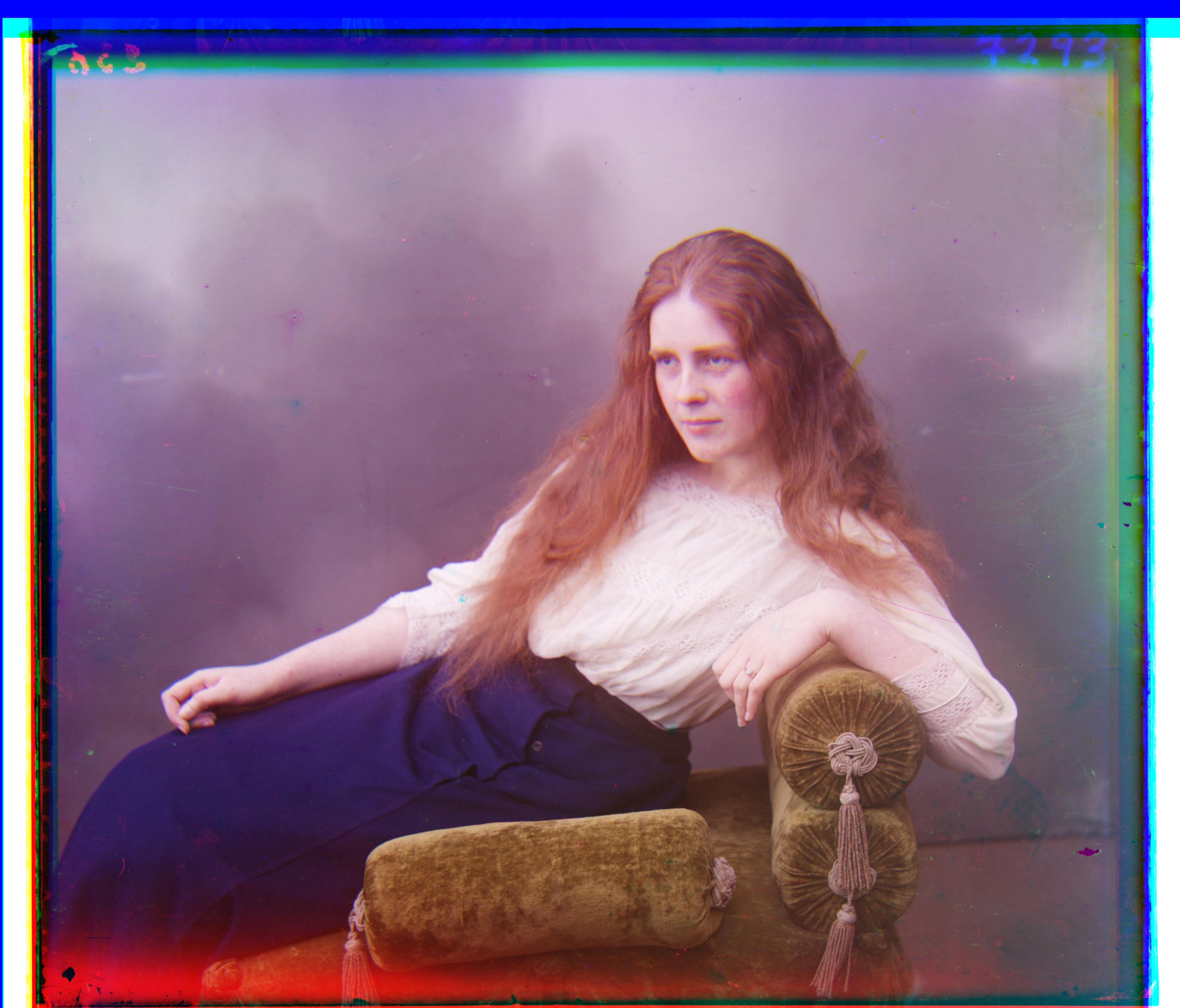
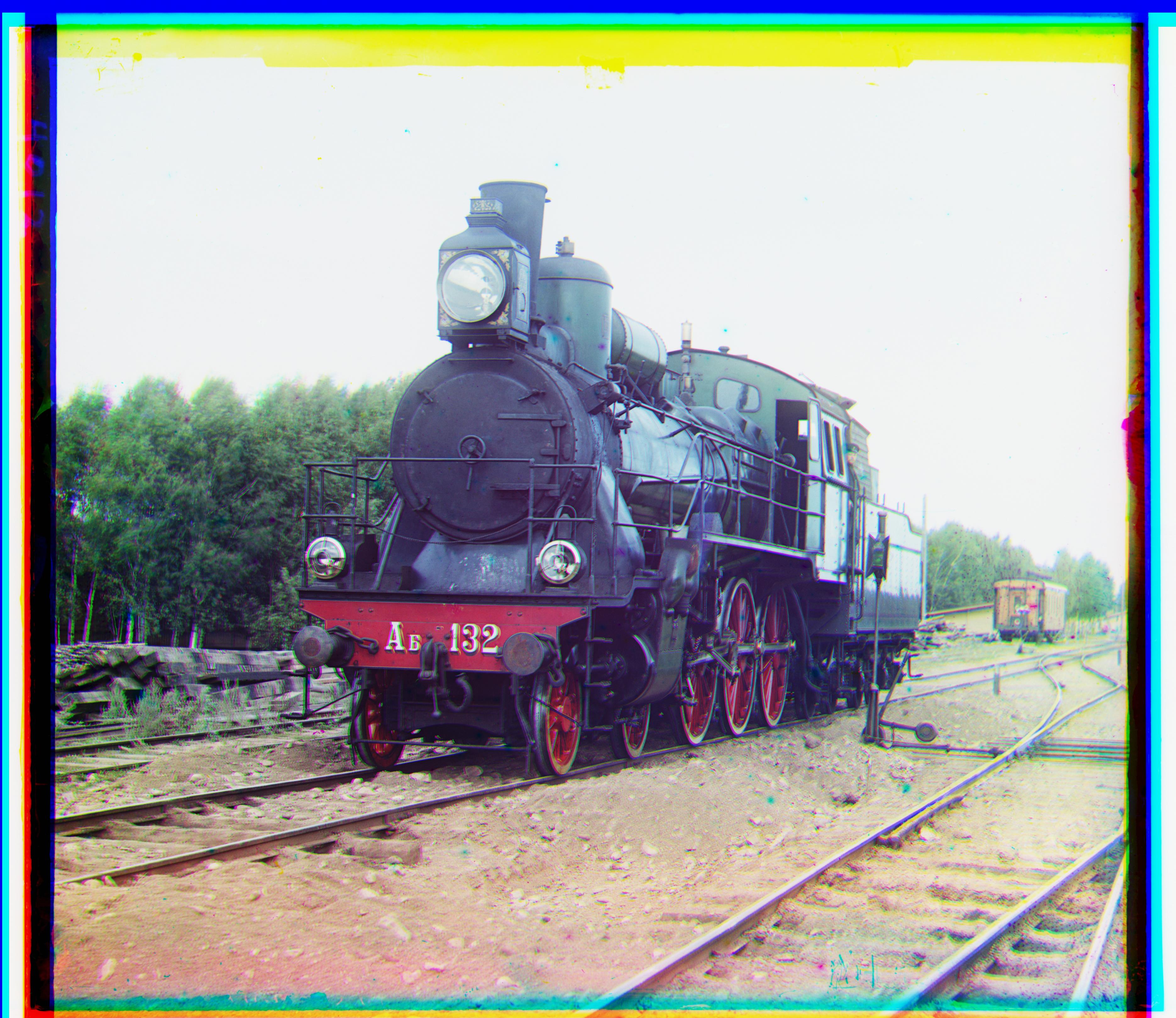
Using image processing techniques, one can convert the stacked images shown above into colorful photographs showcasing the beauty of the Russian Empire in the early 20th century.

Single-scale Alignment

First, I split the starting image into thirds (blue, green, and red). We take the approach of finding displacements for the green and red images and then placing them back on top of the blue image. In order to find the "optimal" displacements of the green and red images, we can choose a metric to score different displacements and then search over as many displacements as possible.

Some possible metrics include Euclidean Distance (L2 norm), Normalized Cross-Correlation (NCC), Structural Similarity Index Measure (SSIM), etc. For this project, we utilize SSIM as implemented in skimage.metrics . Although this metric takes slightly longer to compute than the others, for the larger images, I found this to have better results. Furthermore, I excluded the 5% outside border from the calculation because there is less correlation between the different channels on the borders.

Even on smaller images, it can take awhile to check every possible displacement. Thus, we must intelligently restrict our search space. Notice that some displacements can be ruled out without checking them, as it's likely that the optimal displacement is somewhat close to 0. This is because we assume that the blue, green, and red images are close to each other within a reasonable error. Thus, my algorithm checks a displacement range of [-15, 15] for each of green Δx, green Δy, red Δx, and red Δy.

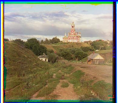
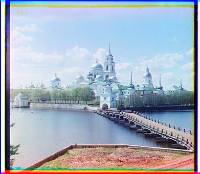
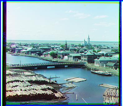
Running this alignment procedure on the three smaller images yields the results shown below.

Multiscale Alignment

For images of a larger scale, the approach described above is infeasible as (1) the scale is larger, so more displacements need to be checked since each pixel is less noticeable and (2) calculating the metric takes longer for each check. Luckily, there is a way to vastly reduce the search space and still maintain a high quality output.

The following is the idea. Recursively scale down the image by a factor of two until a 'small-enough' size is achieved. Then, use the procedure from before to quickly find the 'optimal' displacement of this smaller image. Then, scaling this image up along with the calculated displacement yields a close approximation of the 'optimal' displacement for the higher quality image. Repeat this process until the image returns to its original size.

My algorithm calculates the 'small-enough' size by finding the depth such that smallest side of the image is roughly 100 pixels. Then, it checks a range of [-3, 3] for each displacement. After finding the 'optimal' displacement, I rescale up the current image and the current optimal displacement by a factor of 2. I repeat this process until I return to my original image, where I have to calculate very few displacements since my approximation should already be very close.

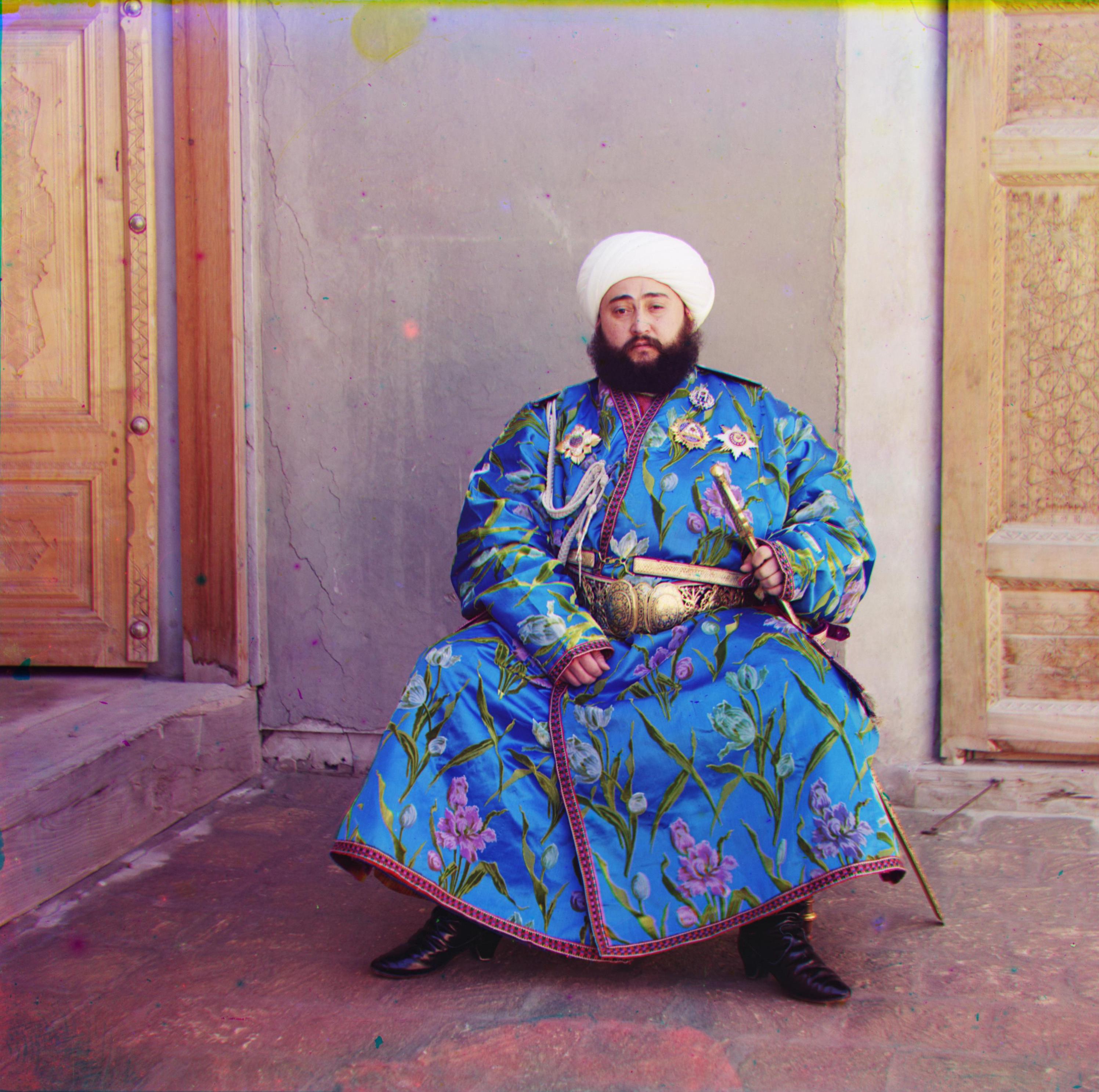
Running this multiscale alignment procedure on the larger images yields the results shown below (in a much faster time than it would take with the single-scale alignment procedure).

Table of Displacements

filename	method	green dx	green dy	red dx	red dy	time
cathedral.jpg	single-scale	5	2	12	3	11.06
monastery.jpg	single-scale	-3	2	3	2	11.19
tobolsk.jpg	single-scale	3	3	6	3	11.09
church.tif	multiscale	25	4	59	-4	107.29
emir.tif	multiscale	50	22	105	40	110.21
harvesters.tif	multiscale	59	15	122	12	118.93
icon.tif	multiscale	39	16	89	23	124.10
lady.tif	multiscale	57	8	120	12	133.33
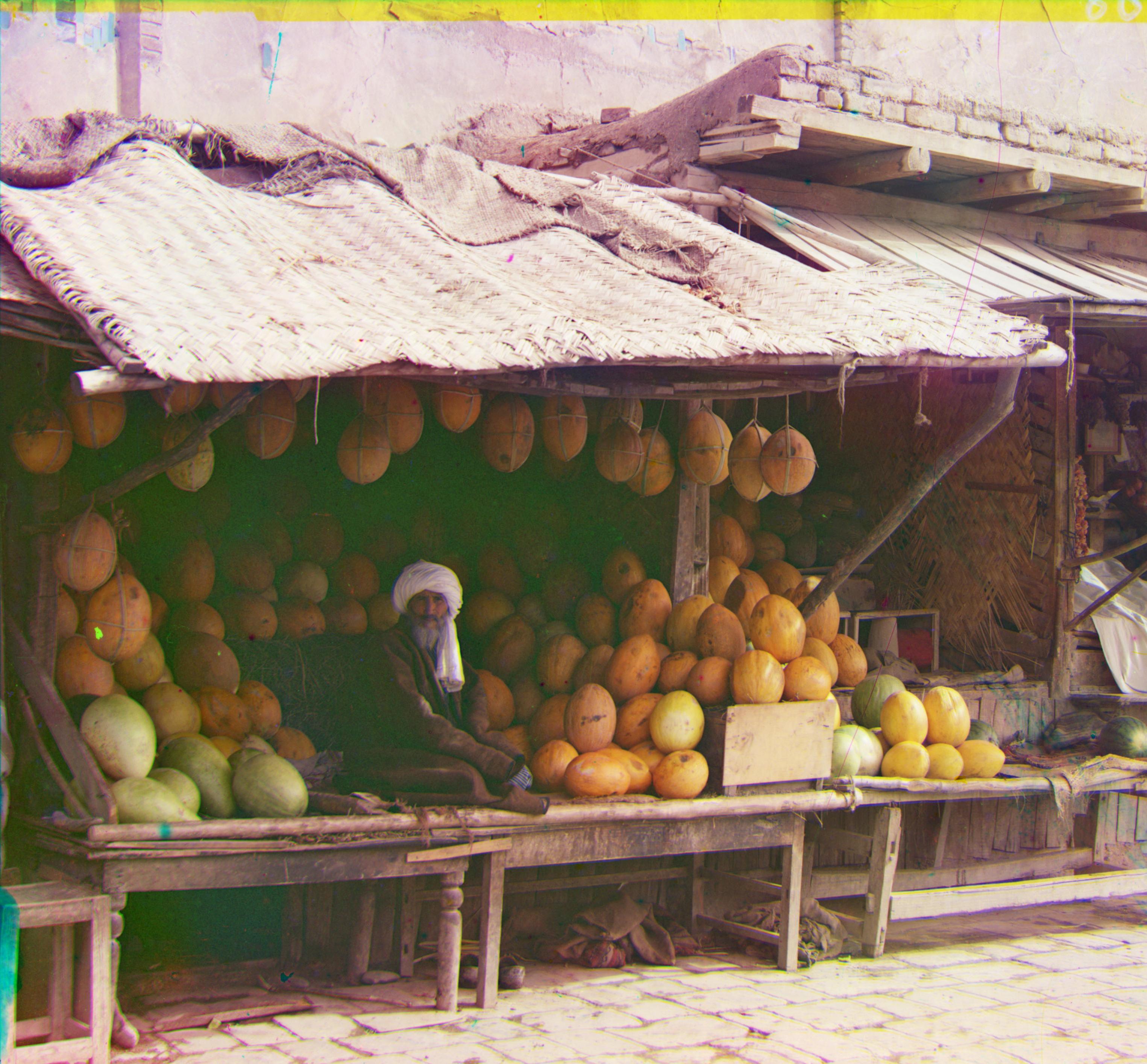
melons.tif	multiscale	80	10	177	13	112.90
onion_church.tif	multiscale	52	25	108	35	123.56
sculpture.tif	multiscale	33	-11	140	-27	140.27
self_portrait.tif	multiscale	78	28	175	37	159.43
three_generations.tif	multiscale	56	17	113	10	111.33
train.tif	multiscale	40	7	85	29	134.13

Bells and Whistles

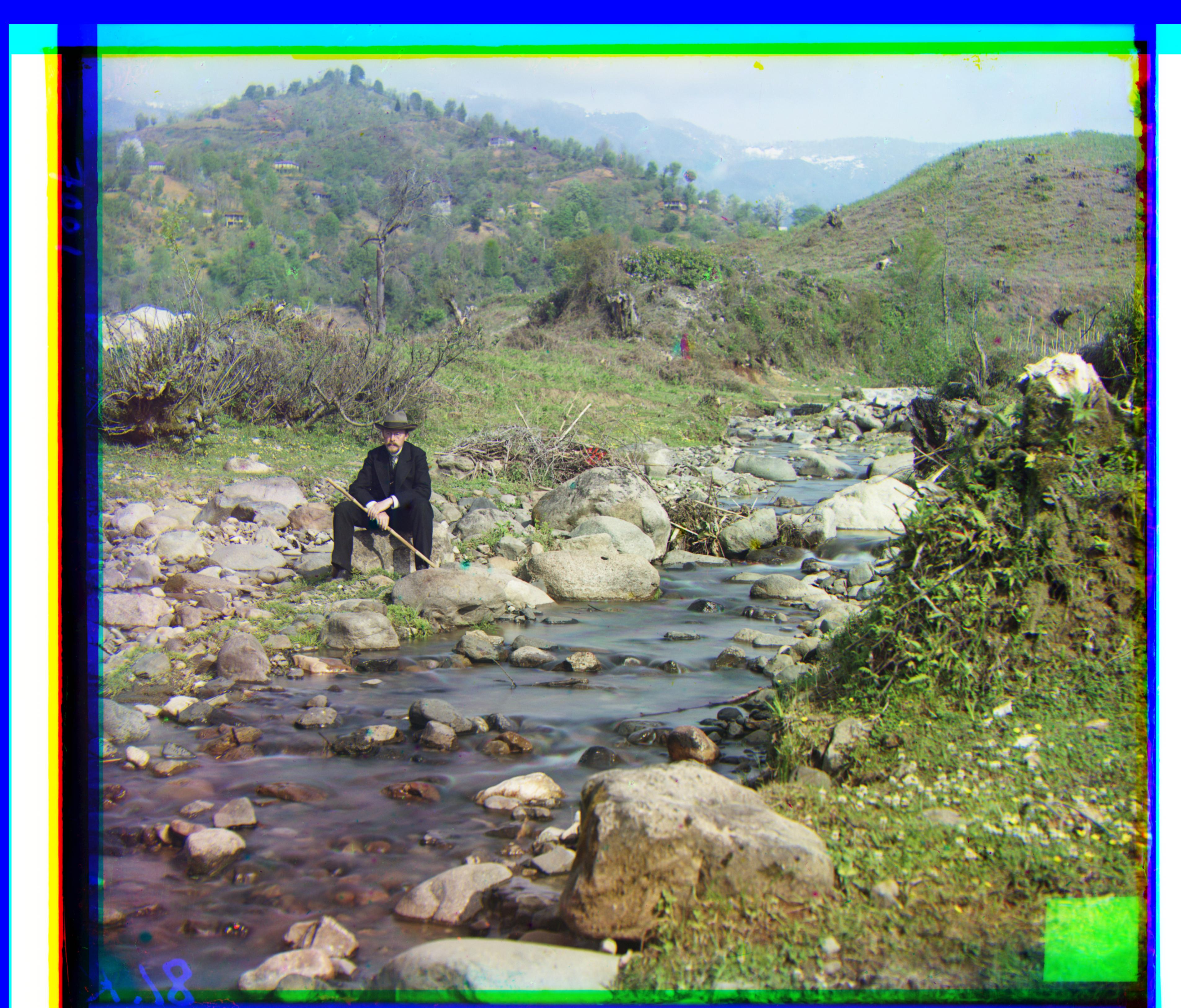
Notice that after the alignment process is complete, each image is left with some borders. As these borders are not the same for each image, some custom border-cropping procedure is needed to clean up the photos (rather than setting a default crop). Thus, I devised the following procedure to automatically crop the aligned photos:

First, use the calculated 'optimal' displacement to make the obvious cuts. For example, if the red channel is shifted to the right by 20 pixels, then clearly the leftmost 20 pixels of the overall image can be safely cut as the lack of red will at the very least create an artificial border (if there isn't already a border there). Since the blue channel stays fixed, any displacement of the green and red channels gives us some safe cuts to make, as we won't want any parts of our picture to not contain all three color channels.

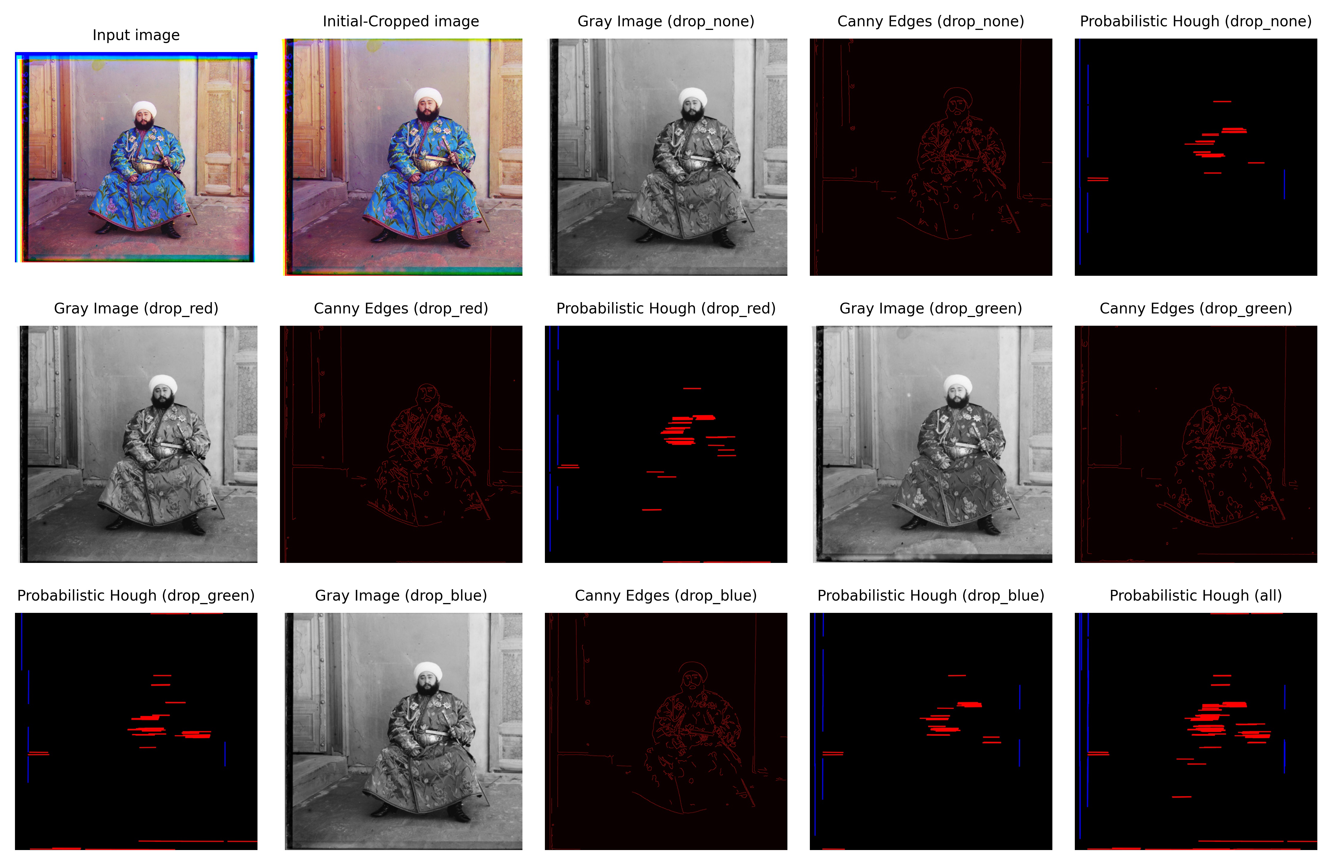
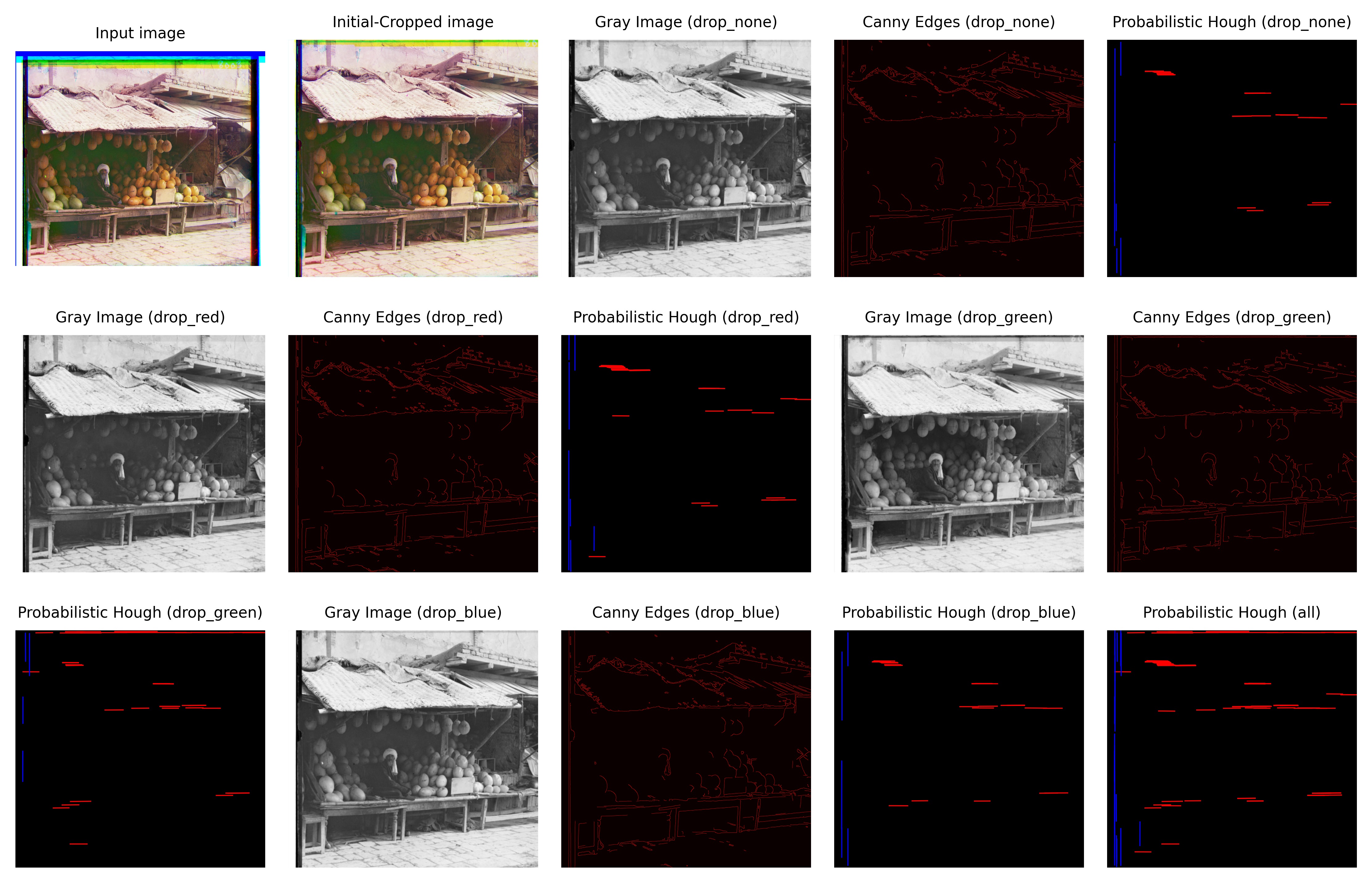
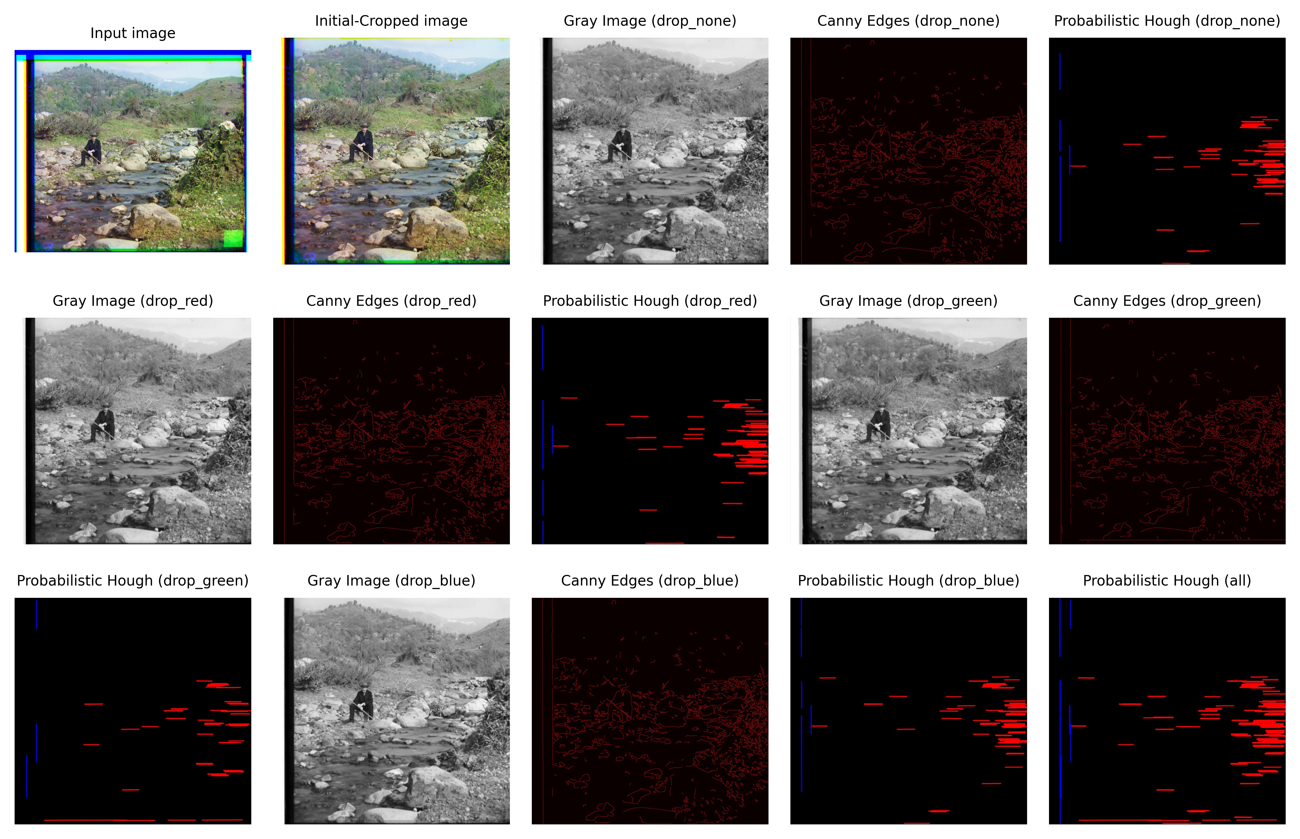
Second, convert the initial crop to grayscale in the following ways: (1) using all color channels along with the weights for each channel specified by skimage.color.rgb2array , (2) dropping the red channel, (3) dropping the green channel, and (4) dropping the blue channel. The reason for dropping channels is we want to be able to detect color edges beyond just black and white, and this is harder to do if we only use a singular gray image.

Third, run Canny edge detection on each grayscale image to get an approximation of the edges present in the image. I used the skimage.feature.canny implementation, with σ=3 and default values for everything else. Without runniny Canny edge detection, the results of the next step were too unpredictable and uncontrolled.

Fourth, run probabilistic Hough transform on the edges from the previous step, checking for vertical and horizontal lines. I used the skimage.transform.probabilistic_hough_line implementation, with threshold=5, line_length=200, line_gap=50 for the horizontal line check and threshold=50, line_length=300, line_gap=25 for the vertical line check. I made the constraints harder on the vertical lines because I found my algorithm struggling more with cropping horizontally than vertically.

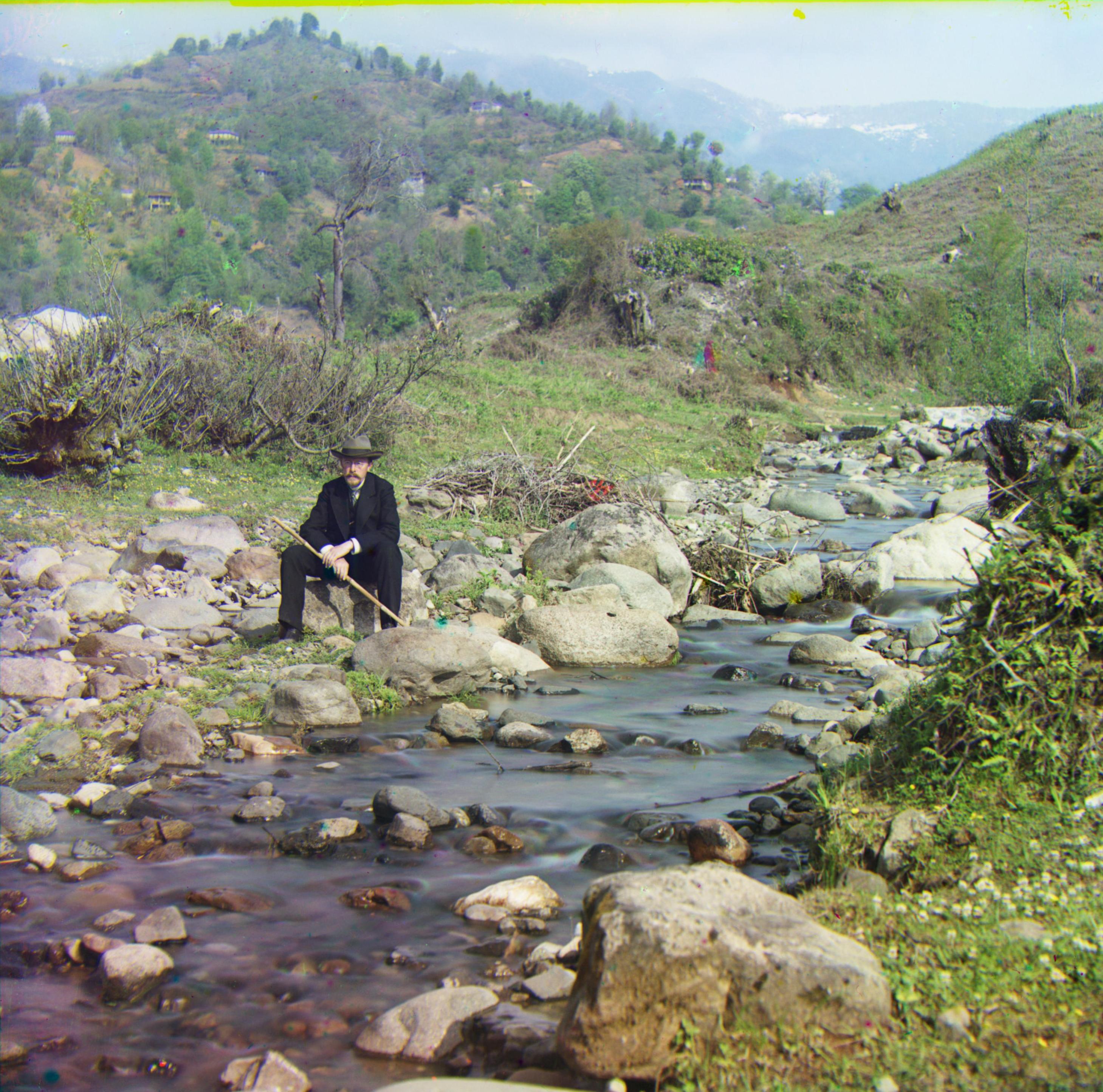
Finally, use the detected lines (all of them from each of the four grayscale images) on the outer 10% of the image to make the final crop. Following this process yielded the following results:

All black and white borders were successfully cropped. Some remnants or partial color borders remained, so my algorithm has room for improvement there. Originally, when I only used the full grayscale image, my algorithm did even worse with the partial color borders, but including the grayscale images with each of the channels removed improved my results significantly.