In this project, I deploy and implement diffusion models,
a type of generative model for images. Diffusion models work by learning learning to remove noise from an
image to move it back onto the natural image manifold.
First, I deploy the
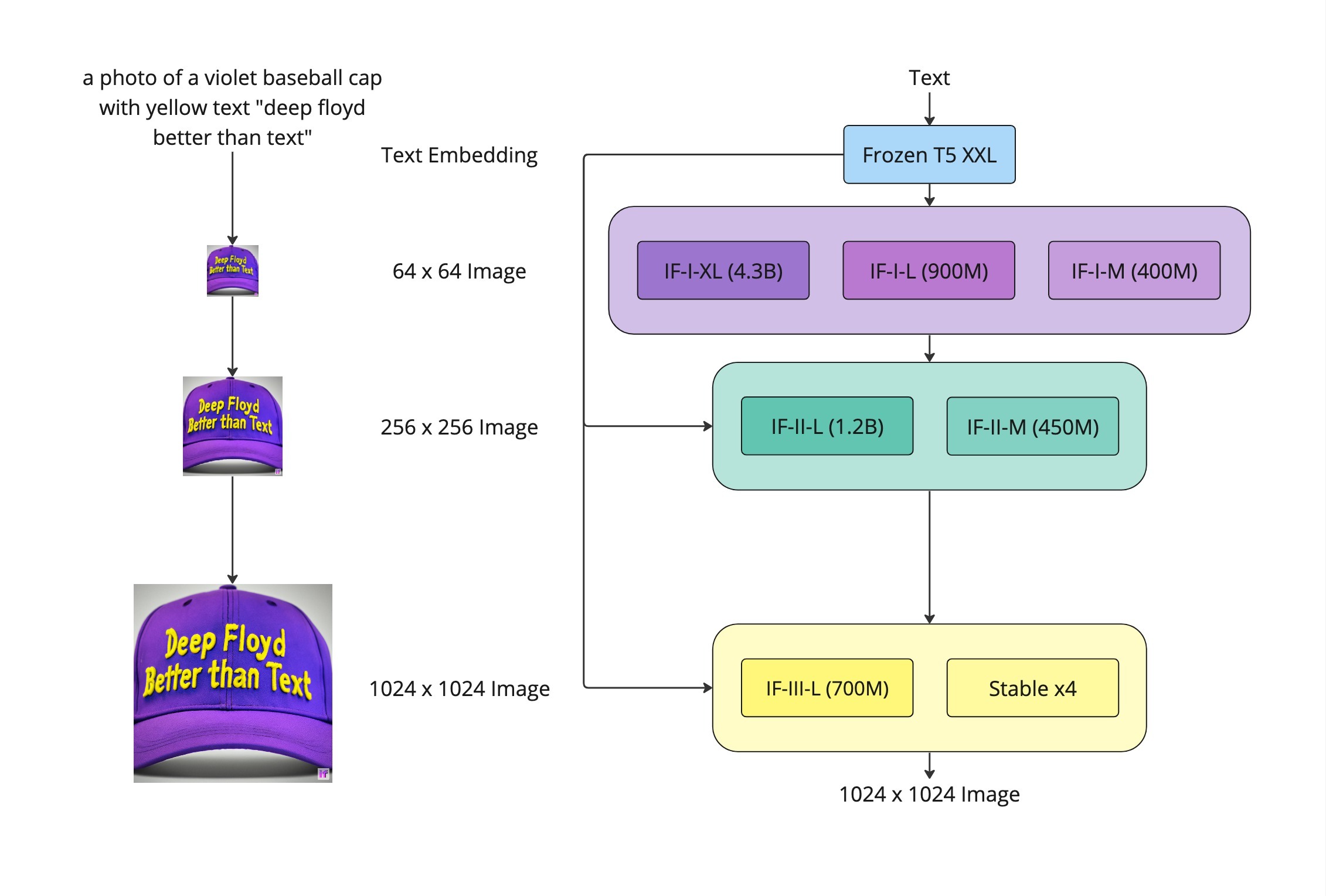
DeepFloyd IF, a diffusion model
trained by Stability AI. Using this model, I showcase the capabilities
of diffusion models by demonstrating sampling, denoising, image-to-image translation, inpainting, visual
anagrams, and hybrid images.
Second, I implement a diffusion model from scratch
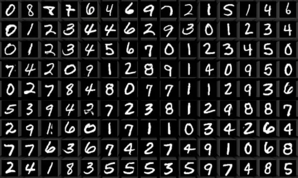
to generate handwritten digits by training on the MNIST dataset.
I utilize the UNet architecture to implement models capable of
one-step denoising and diffusion (with time and class conditiong). I also implement sampling with
classifer-free guidance (CFG) to improve the results of the
generated images.
Part A: The Power of Diffusion Models!
Part 0: Setup
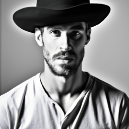
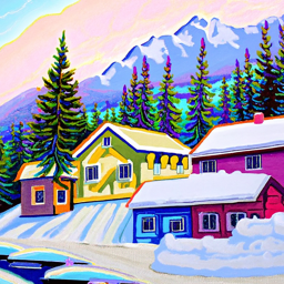
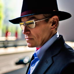
First, we load the DeepFloyd IF diffusion model from Hugging Face. Since DeepFloyd was trained as a text-to-image model, we also need to load some precomputed text embeddings. Among those is the embedding for the prompt "a high quality photo", which I will later use as a pseudo-null prompt. For now, we test the model on three other prompts. Note that the model has multiple stages, which output images at progressively higher resolutions. For now, we use the first two stages, but later on we will just use the first stage.

(stage 1, num_inference_steps=20)

(stage 1, num_inference_steps=20)

(stage 1, num_inference_steps=20)
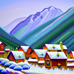
(stage 2, num_inference_steps=20)
(stage 2, num_inference_steps=20)

(stage 2, num_inference_steps=20)
The above images were sampled with 20 inference steps. This means that the diffusion model was run 20 times for each image. During the training of DeepFloyd, the noising/denoising process was split into $T=1000$ steps, but it turns out that during inference, we can get away with significantly reducing the number of steps. That being said, decreasing the number of steps too much can reduce the quality, as it gives less opportunity for fine details to be accounted for. The following were generated with the same prompts, but with twice the number of inference steps, and seem to be of much higher quality.

(stage 1, num_inference_steps=40)

(stage 1, num_inference_steps=40)

(stage 1, num_inference_steps=40)
(stage 2, num_inference_steps=40)
(stage 2, num_inference_steps=40)

(stage 2, num_inference_steps=40)
Part 1: Sampling Loops
1.1 Implementing the Forward Process
The forward process is a key part of diffusion. This is the process by a which a clean image
is turned into noise. The following defines the forward process:
$$q(x_t\mid x_0)=\mathcal{N}(x_t;\sqrt{\bar{\alpha}}x_0,(1-\bar{\alpha}_t)\mathbf{I})$$
This is equivalent to computing $x_t=\sqrt{\bar{\alpha}_t}x_0+\sqrt{1-\bar{\alpha}_t}\epsilon$
where $\epsilon\sim\mathcal{N}(0, 1)$. Note that $t=0$ corresponds to the clean image and larger
values of $t$ correspond to larger amounts of noise being injected into the image.
Using the scheduler from the first stage of DeepFloyd, we can recover the values of $\bar{\alpha}_t$
for $t\in[0,999]$. Using these values, we can visualize the forward process on a familiar tower.
1.2 Classical Denoising
Suppose we are given a noisy image and wish to denoise it using strictly classical methods. Using Gaussian blur filtering, we can attempt to remove some noise, though we will later see that diffusion models do a much better job. The following are attempts at denoising the noisy images using this technique:

$(t=250)$

$(t=500)$

$(t=750)$

$(t=250)$

$(t=500)$

$(t=750)$
1.3 One-Step Denoising
Next, we'll try to use diffusion models to denoise the noisy images. While classical methods
are unable to recover lost information, machine-learning-based methods are able to utilize their
training from a vast set of images to hallucinate information and project onto the natural image
manifold.
As discussed earlier, we use the embedding for the prompt "a high quality photo" as conditioning for
the model. The following are the one-step denoising results:

$(t=250)$

$(t=500)$

$(t=750)$

$(t=250)$

$(t=500)$

$(t=750)$
1.4 Iterative Denoising
While this performs much better than the classical method, it does get worse as more noise is added.
This makes sense as the problem is harder and diffusion models are designed to iteratively denoise
rather than doing it all in one step.
While this diffusion model was trained on $T=1000$ denoising steps, we can actually skip steps
as mentioned earlier. We do this by denoising from $t=990$ to $t=0$ with a stride of $30$. That is,
we consider the following values of $t$: $990,960,930,\ldots,60,30,0$.
To denoise, we implement the following formula:
$$x_{t'}=\frac{\sqrt{\bar{\alpha}_{t'}}\beta_t}{1-\bar{\alpha}_t}x_0+
\frac{\sqrt{\alpha_t}(1-\bar{\alpha}_{t'})}{1-\bar{\alpha}_t}x_t + v_\sigma,$$
where $t$ is the current timestep, $t'$ is the
next timestep, $\bar{\alpha}_t$ is as explained above, $x_t$ is the current noisy image,
$x_{t'}$ is the (less) noisy image at timestep $t'$, $\alpha_t=\frac{\bar{\alpha}_t}{\bar{\alpha}_{t'}}$,
$\beta_t=1-\alpha_t$, and $v_\sigma$ is random noise (in this case predicted by DeepFloyd).
Starting at $t=690$, we get the following results for iterative denoising, one-step denoising,
and Gaussian blur denoising:

$(t=690)$

$(t=540)$

$(t=390)$

$(t=240)$

$(t=90)$

$(t=0)$

$(t=690)$

$(t=690)$

1.5 Diffusion Model Sampling
Using the same procedure defined above, we can generate images from scratch rather than just denoising an image. By passing in complete noise, we can denoise pure noise to generate new images. Doing this yields the following:


1.6 Classifier-Free Guidance (CFG)
The quality of the above images leaves a lot of room for improvement. One easy way
to improve the quality is to use a technique known as classifer-free guidance (CFG).
In CFG, we compute conditional and unconditional noise estimates, denoted by
$\epsilon_c$ and $\epsilon_u$ respectively. We then define our new noise estimate by
the following:
$$\epsilon_{CFG}=\epsilon_u+\gamma(\epsilon_c - \epsilon_u),$$
where $\gamma$ is a hyperparameter that controls the strength of CFG. Intuitively,
$\epsilon_{CFG}$ can be thought of as noise moving more in the direction
of the condition given to the model. To get $\epsilon_c$, we use the embedding for the prompt "a high quality photo" and to
get $\epsilon_u$, we use the embedding for the empty string.
The following were generated using CFG with $\gamma=7$:


1.7 Image-to-Image Translation
In 1.4, we took an image, added noise to it, and then denoised it. This allowed us to make edits to a preexisting image. Here, we do this again, this time using CFG. This follows the SDEdit algorithm. The following showcases this process, with $i_{\text{start}}\in\{1,3,5,7,10,20\}$, where larger $i_{\text{start}}$ means less noise to start with.

with $i_{\text{start}}=1$

with $i_{\text{start}}=3$

with $i_{\text{start}}=5$

with $i_{\text{start}}=1$

with $i_{\text{start}}=10$

with $i_{\text{start}}=20$


with $i_{\text{start}}=1$

with $i_{\text{start}}=3$

with $i_{\text{start}}=5$

with $i_{\text{start}}=1$

with $i_{\text{start}}=10$

with $i_{\text{start}}=20$


with $i_{\text{start}}=1$

with $i_{\text{start}}=3$

with $i_{\text{start}}=5$

with $i_{\text{start}}=1$

with $i_{\text{start}}=10$

with $i_{\text{start}}=20$

1.7.1 Editing Hand-Drawn and Web Images
Repeating this process on hand-drawn images yields the following:

with $i_{\text{start}}=1$

with $i_{\text{start}}=3$

with $i_{\text{start}}=5$

with $i_{\text{start}}=1$

with $i_{\text{start}}=10$

with $i_{\text{start}}=20$


with $i_{\text{start}}=1$

with $i_{\text{start}}=3$

with $i_{\text{start}}=5$

with $i_{\text{start}}=1$

with $i_{\text{start}}=10$

with $i_{\text{start}}=20$

Repeating this process on an image drawn from the web yields the following:

with $i_{\text{start}}=1$

with $i_{\text{start}}=3$

with $i_{\text{start}}=5$

with $i_{\text{start}}=1$

with $i_{\text{start}}=10$

with $i_{\text{start}}=20$

1.7.2 Inpainting
The above procedure makes edits to the entire image. Suppose we just want to change
part of the image. This (inpainting) is also possible with diffusion models. Following
the RePaint paper, we can perform inpainting by
repeating the above procedure but forcing $x_t$ to have the same pixels as our original image
wherever we don't want things to change.
That is, suppose we are given an image $x_{\text{orig}}$ and binary mask $\mathbf{m}$. We create
a new image that has the same content as $x_{\text{orig}}$ wherever $\mathbf{m}$ is $0$ and new
content wherever $\mathbf{m}$ is $1$. We accomplish this by setting $x_t$ to $x_{\text{orig}}$
wherever $\mathbf{m}$ is 0 after every step, as described by the following:
$$x_t\leftarrow \mathbf{m}x_t + \text{forward}(x_{\text{orig}}, t)$$
Performing this procedure yeilds the following:


1.7.3 Text-Conditional Image-to-Image Translation
Next, we run the SDEdit algorithm again, but this time with prompts other than "a high quality photo". The results along with their corresponding prompts are shown below:

on Campanile
with $i_{\text{start}}=1$

on Campanile
with $i_{\text{start}}=3$

on Campanile
with $i_{\text{start}}=5$

on Campanile
with $i_{\text{start}}=1$

on Campanile
with $i_{\text{start}}=10$

on Campanile
with $i_{\text{start}}=20$


old man on Ryan
with $i_{\text{start}}=1$

old man on Ryan
with $i_{\text{start}}=3$

old man on Ryan
with $i_{\text{start}}=5$

old man on Ryan
with $i_{\text{start}}=1$

old man on Ryan
with $i_{\text{start}}=10$

old man on Ryan
with $i_{\text{start}}=20$


on Cat
with $i_{\text{start}}=1$

on Cat
with $i_{\text{start}}=3$

on Cat
with $i_{\text{start}}=5$

on Cat
with $i_{\text{start}}=1$

on Cat
with $i_{\text{start}}=10$

on Cat
with $i_{\text{start}}=20$

1.8 Visual Anagrams
Next, we implement Visual Anagrams,
creating optical optical illusions with diffusion models. Specifically, we create
images which appear like different things when flipped. To do this, we obtain noise
estimates for two prompts, but with one of them flipped.
That is, suppose we have two prompts $p_{up},p_{down}$. We obtain our noise estimate $\epsilon$ by
the following:
$$\epsilon_{up}=\text{UNet}(x_t,t,p_{up})$$
$$\epsilon_{down}=\text{flip}(\text{UNet}(\text{flip}(x_t),t,p_{down}))$$
$$\epsilon=(\epsilon_{up}+\epsilon_{down}) / 2$$
Note that we can also run CFG on each of $\epsilon_{up},\epsilon_{down}$ to further
improve the results. Implementing all of this yields the following results:

down: an oil painting of an old man
Sample 1

down: an oil painting of an old man
Sample 2

down: an oil painting of an old man
Sample 3

down: a photo of the amalfi cost
Sample 1

down: a photo of the amalfi cost
Sample 2

down: a photo of the amalfi cost
Sample 3

down: a photo of a dog
Sample 1

down: a photo of a dog
Sample 2

down: a photo of a dog
Sample 3
1.9 Hybrid Images
Using a similar idea, we can implement Factorized Diffusion
to create hybrid images. That is, we can create a composite noise estimate by estimating the noise
of different prompts, then combining low frequencies of one noise with high frequencies of the other.
That is, suppose we have two prompts $p_{low},p_{high}$. For $f_{\text{lowpass}},f_{\text{highpass}}$
being lowpass and higpass filters respectively, we obtain our noise estimate $\epsilon$ by the following:
$$\epsilon_{low}=\text{UNet}(x_t,t,p_{low})$$
$$\epsilon_{high}=\text{UNet}(x_t,t,p_{high})$$
$$\epsilon=f_{\text{lowpass}}(\epsilon_{low})+f_{\text{highpass}}(\epsilon_{high})$$
As before, we can run CFG on $\epsilon_{low},\epsilon_{high}$ to further improve the results.
Implementing all of this yields the following results:

high: a lithograph of waterfalls
Sample 1

high: a lithograph of waterfalls
Sample 2

high: a lithograph of waterfalls
Sample 3

high: a man wearing a hat
Sample 1

high: a man wearing a hat
Sample 2

high: a man wearing a hat
Sample 3

high: a rocket ship
Sample 1

high: a rocket ship
Sample 2

high: a rocket ship
Sample 3
Part B: Diffusion Models from Scratch!
...
Part 1: Training a Single-Step Denoising UNet
We start by training a simple one-step denoiser. That is, given a noisy image $z$, we train a model $D_\theta$ to map $z$ to a clean image $x$. We do so by optimizing over L2 loss: $$L=\mathbb{E}_{z,x}\|D_\theta(z)-x\|^2$$ Note that at this stage, $D_\theta$ is not conditioned on time or class. It's only goal is to denoise an image back onto the image manifold. Conditioning will come later.
1.1 Implementing the UNet
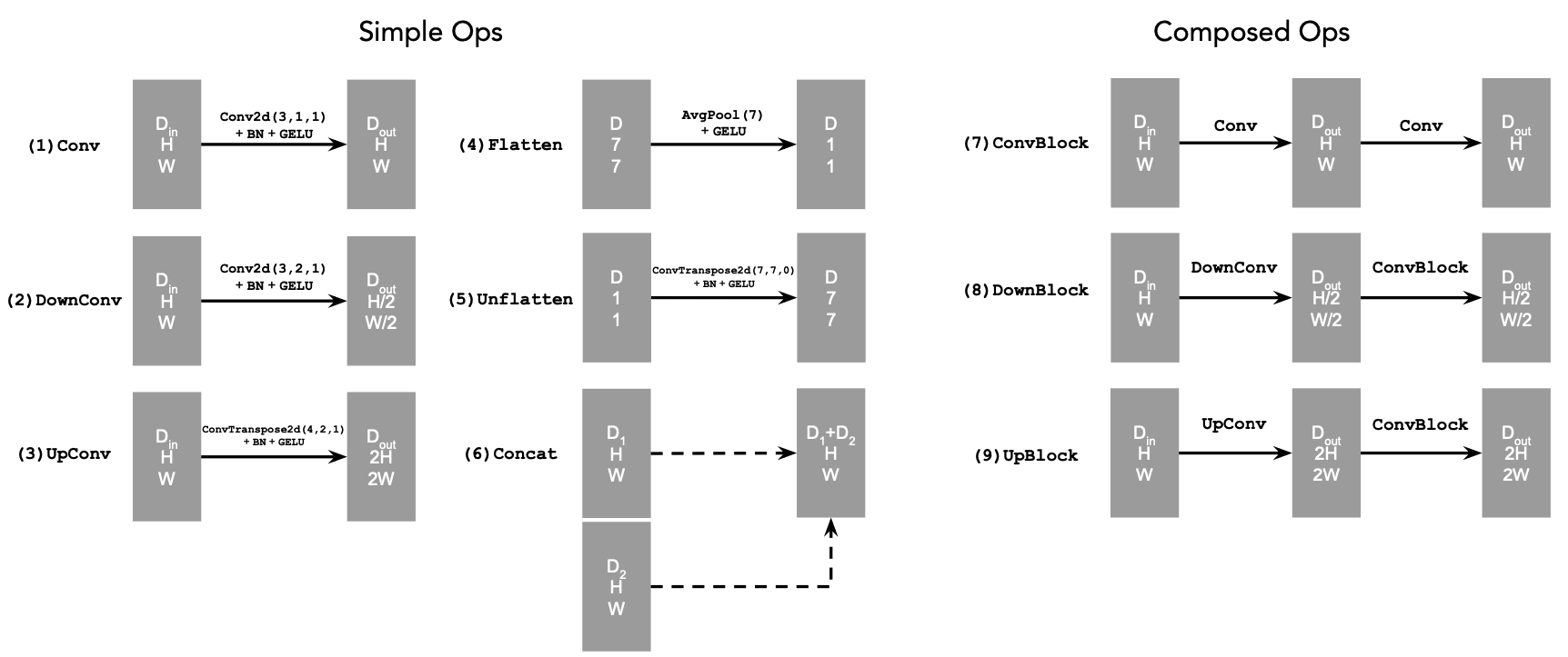
We implement our denoiser model $D_\theta$ as a UNet, consisting of downsampling and upsampling blocks with skip connections. The following diagram showcases the architecture of our model:
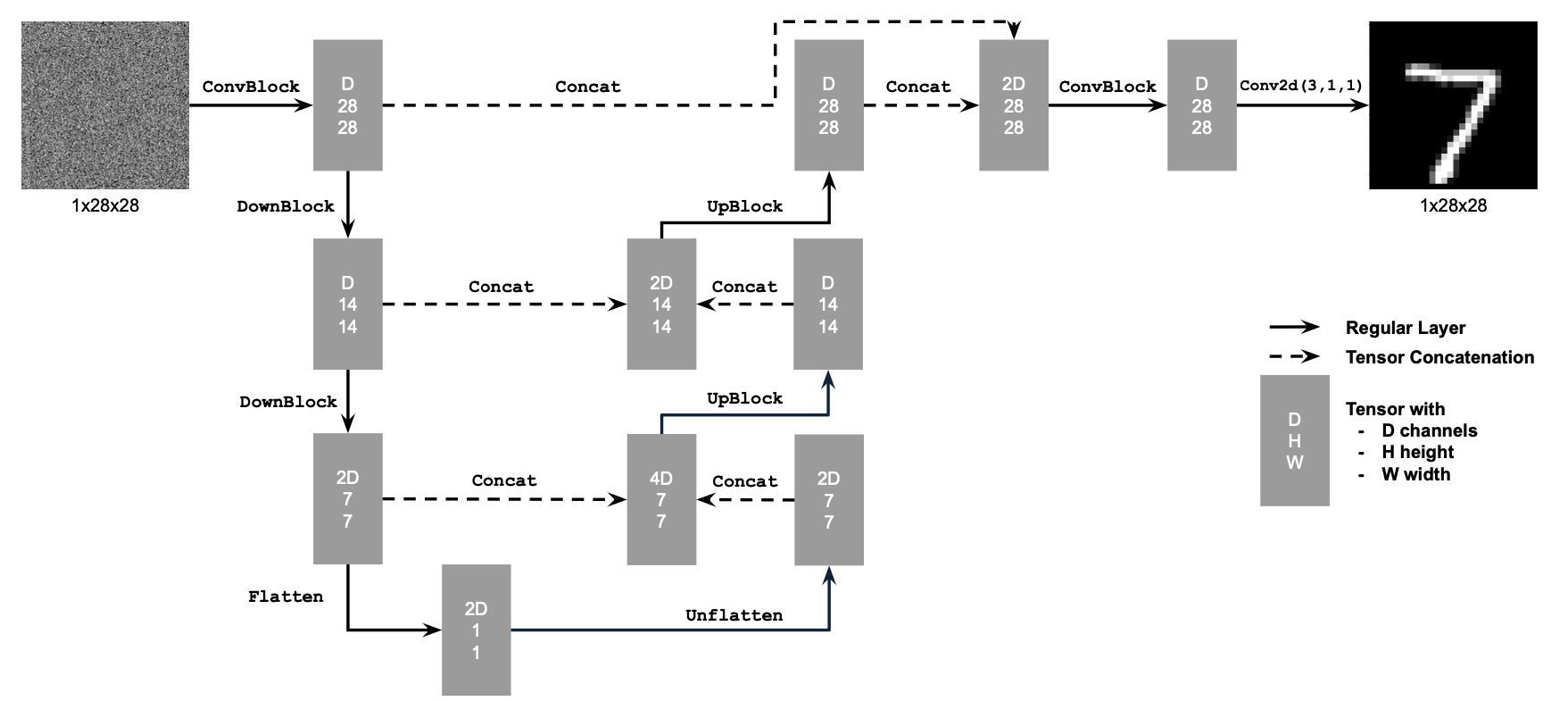
The operations of the diagram above are further decomposed into simpler tensor operations as follows:
1.2 Using the UNet to Train a Denoiser
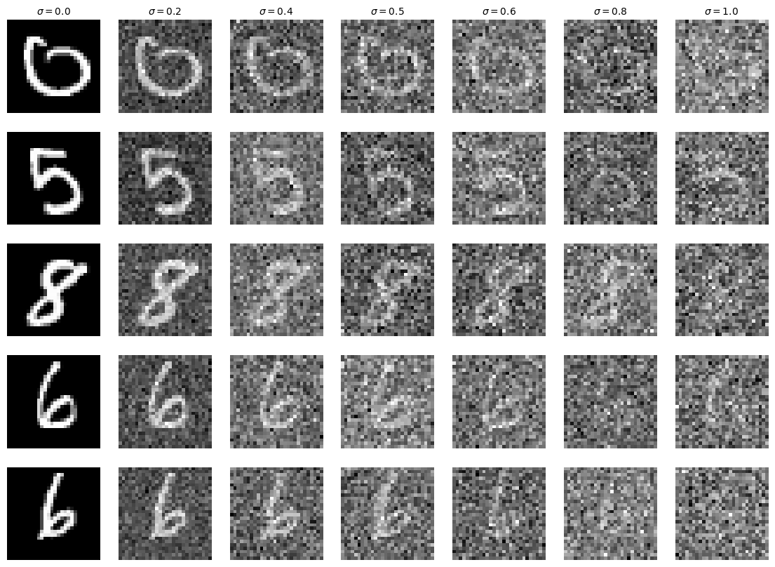
In order to train $D_\theta$, we must generate pairs $(z,x)$, where $x$ is sampled from the MNIST dataset and $z$ is a noised version of $x$. For each training batch, we generate $z$ from $x$ using the following noising process: $$z=x+\sigma\epsilon,$$ where $\epsilon\sim\mathcal{N}(0,1)$ and $\sigma$ is chosen by us. The following showcases the results of this noising process for different values of $\sigma$:
1.2.1 Training
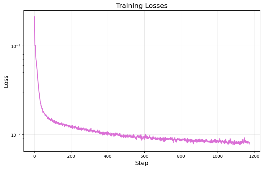
Now we are ready to train our denoiser $D_\theta$. We train on noisy images corresponding to $\sigma=0.5$, use a batch size of $256$ for $5$ epochs, define our model with a hidden dimension $D=128$, and use the Adam optimizer with a fixed learning rate of $0.0001$. Doing so yields the following training loss curve:
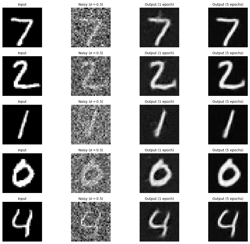
Visualizing the denoised results on the test set for the model after the first and fifth epoch, we see the following:
1.2.2 Out-of-Distribution Testing
While our denoiser $D_\theta$ was trained on digits noised with $\sigma=0.5$, we can still test on other values of $\sigma$. The following showcases the denoiser results on a test set digit with varying levels of noise applied to it.

Part 2: Training a Diffusion Model
Now we move away from one-step denoising and towards diffusion. We utilize our UNet architecture
from the previous section to implement DDPM. We
change our UNet to predict the added noise $\epsilon$ rather than the clean image $x$. Thus, our
loss becomes the following:
$$L=\mathbb{E}_{z,\epsilon}\|\epsilon_\theta(z)-\epsilon\|^2,$$
where $\epsilon_\theta$ is a UNet trained to predict noise. Since we are doing diffusion,
we will eventually want to sample pure noise $\epsilon\sim\mathcal{N}(0,1)$ and generate
a realistic image $x$. However, as seen before, the capability of one-step denoising is
limited, so we instead focus on iterative denoising.
We use the following equation from before to generate noisy images $x_t$ from $x_0$
for some timestep $t\in\{0,1,\ldots,T\}$:
$$x_t=\sqrt{\bar{\alpha}_t}x_0+\sqrt{1-\bar{\alpha}_t}\epsilon,$$
where $\epsilon\sim\mathcal{N}(0,1)$. The derivation of $\bar{\alpha}$ is given in the DDPM
paper, but for now we just use the following simplified recipe:
- instantiate a list $\beta$ of length $T$ such that $\beta_0=0.0001$, $\beta_T=0.02$, and $\beta_t$ is evenly spaced between the two for $t\in\{1,2,\ldots,T-1\}$.
- $\alpha_t=1-\beta_t$ for all $t$
- $\bar{\alpha}_t=\prod_{s=1}^t\alpha_t$, the cumulative product of $\alpha_s$ for $s\in\{1,2,\ldots,t\}$
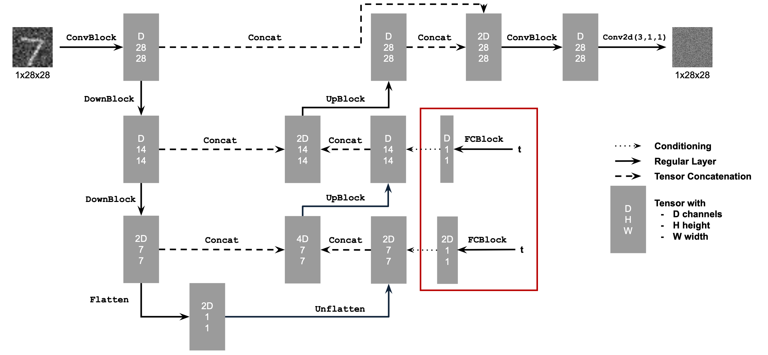
2.1 Adding Time Conditioning to UNet
The following showcases the updated architecture, with conditioning on $t$:

2.2 Training the UNet
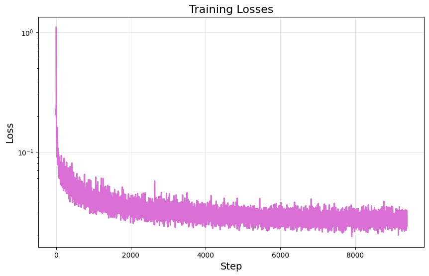
Now we are ready to train our time-conditioned UNet, $\epsilon_\theta(x_t|t)$. We use a batch size of $128$ for $20$ epochs, define our model with hidden dimension $D=64$, and use the Adam optimizer with initial learning rate of $0.001$ and exponential learning rate decay of $0.1^{0.05}$. Doing so yields the following training loss curve:
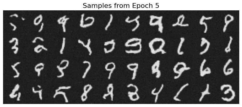
2.3 Sampling from the UNet
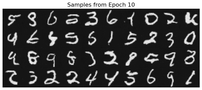
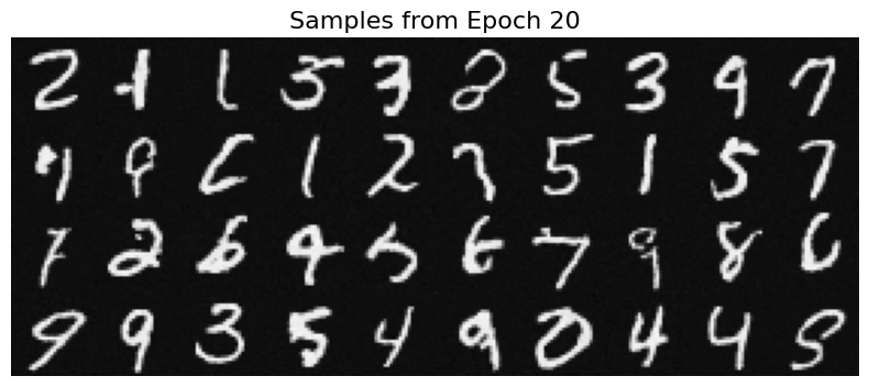
Next, we can sample from our diffusion model just as we did in part A. This yields the following for different epochs: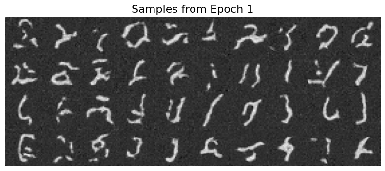
2.4 Adding Class-Conditioning to UNet
We can also add class conditioning to our model by further conditioning on the label during training. During training, we occasionally drop our class conditioning in order to maintain the ability to unconditionally generate images. The following is the training loss curve of our new UNet diffusion model, $\epsilon_\theta(x_t|t,c)$: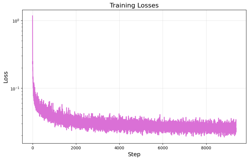
2.5 Sampling from the Class-Conditioned UNet
Sampling from this model, now using CFG as described before, yields the following results: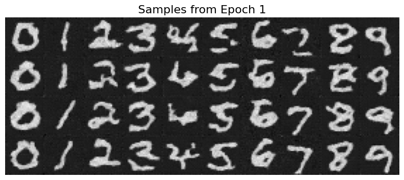
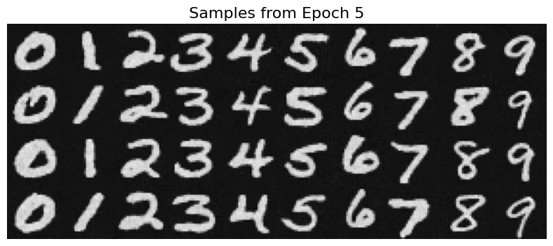
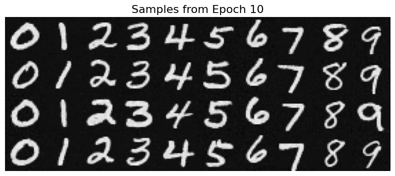
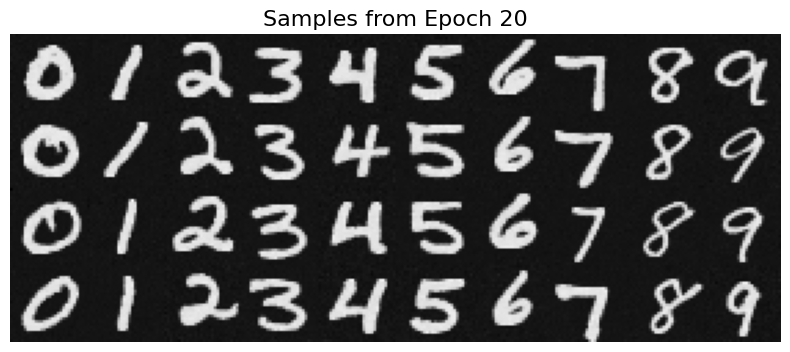
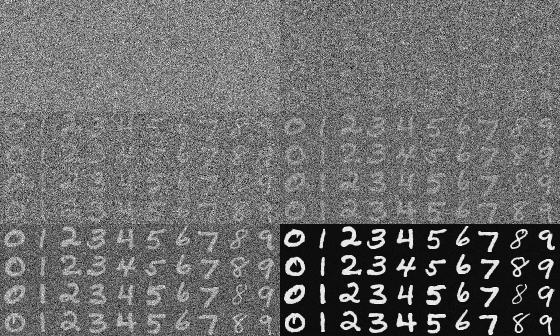
Furthermore, we can visualize the iterative denoising process as follows:
