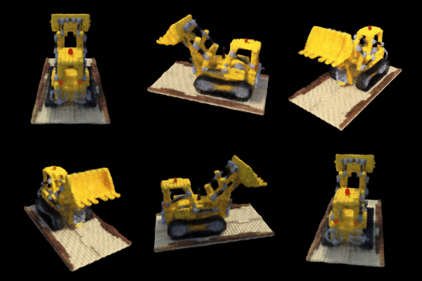
In this project, we implement and train a Neural Radiance Field (NeRF). NeRFs are mappings $F:\{x,y,z,\theta,\phi\}\to\{r,g,b,\sigma\}$ that are used to represent a 3D space. Before implementing NeRFs, we gain some intuition by implementing a Radiance Field in 2D, a mapping $F:\{u,v\}\to\{r,g,b\}$. In order to learn these mappings, we utilize machine learning techniques with neural networks.

Part 1: Fit a Neural Field to a 2D Image
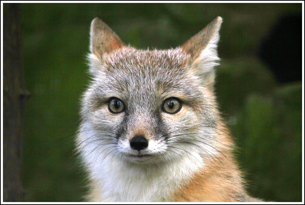
We start by attempting to learn reconstructions of the following images:


In order to do so, we utilize a Multilayer Perceptron (MLP) network with Sinusoidal Positional Encoding (PE) that takes in the 2D pixel coordinates, and output the 3D pixel colors. The following is the architecture that we implement:

PE is an operation in which that you apply a series of sinusoidal functions to the input cooridnates
to expand its dimensionality. It is defined as follows:
$$PE(x, L)=\left[x,\sin(2^0\pi x),\cos(2^0\pi x),\sin(2^1\pi x),\cos(2^1\pi x),\ldots
\sin(2^{L-1}\pi x),\cos(2^{L-1}\pi x)\right]$$
In order to train our MLP, we implement a dataloader, which randomly samples $N$ pixels
each iteration of training. This dataloader provides the training loop with the $N\times 2$ coordinates
and $N\times 3$ colors which are the input and targets of the network respectively.
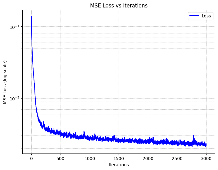
Training with L=10, Adam with a learning rate of 1e-2, a batch size of 10k yields,
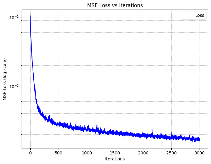
and on MSE loss yields the following training curves:
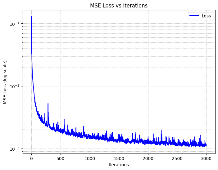
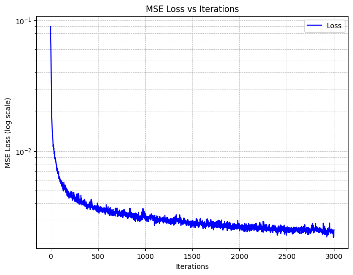
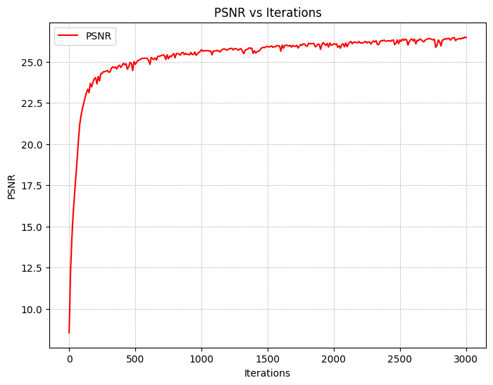
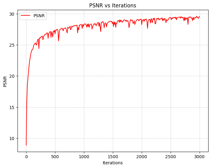
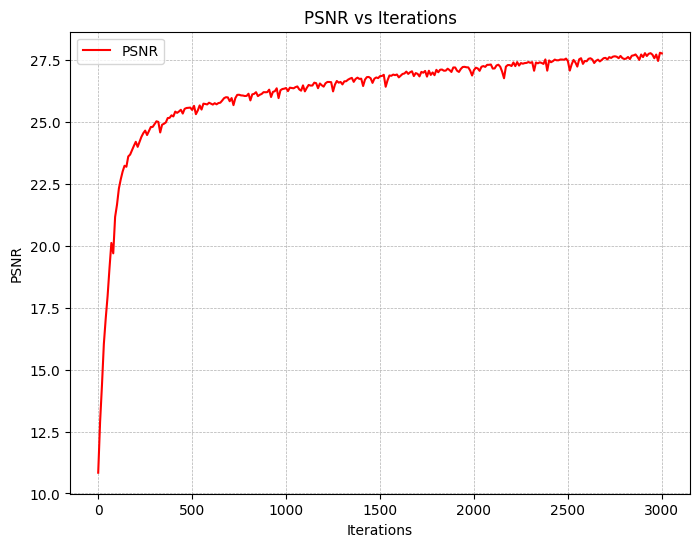
We also utilize Peak Signal-to-Noise Ratio (PSNR) as a metric for measuring the reconstruction quality of the images. This is shown below:
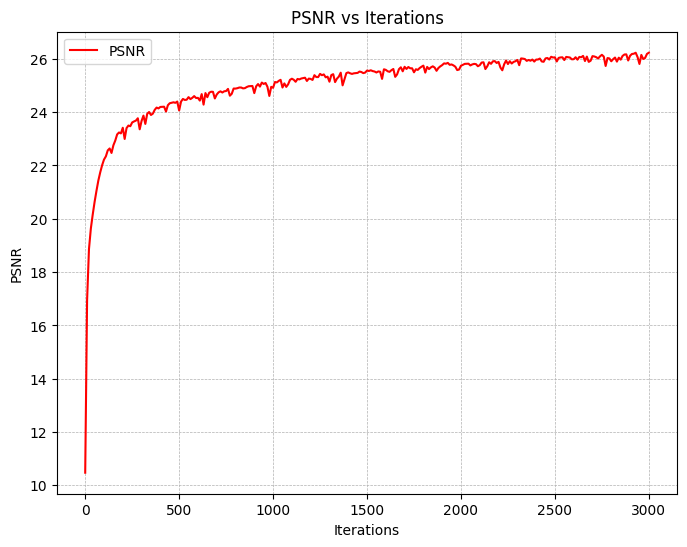
Plotting the predicted images across iterations, we get the following results:


[Bells & Whistles] We can also visualzie the training process by organizing the predicted images into a gif.
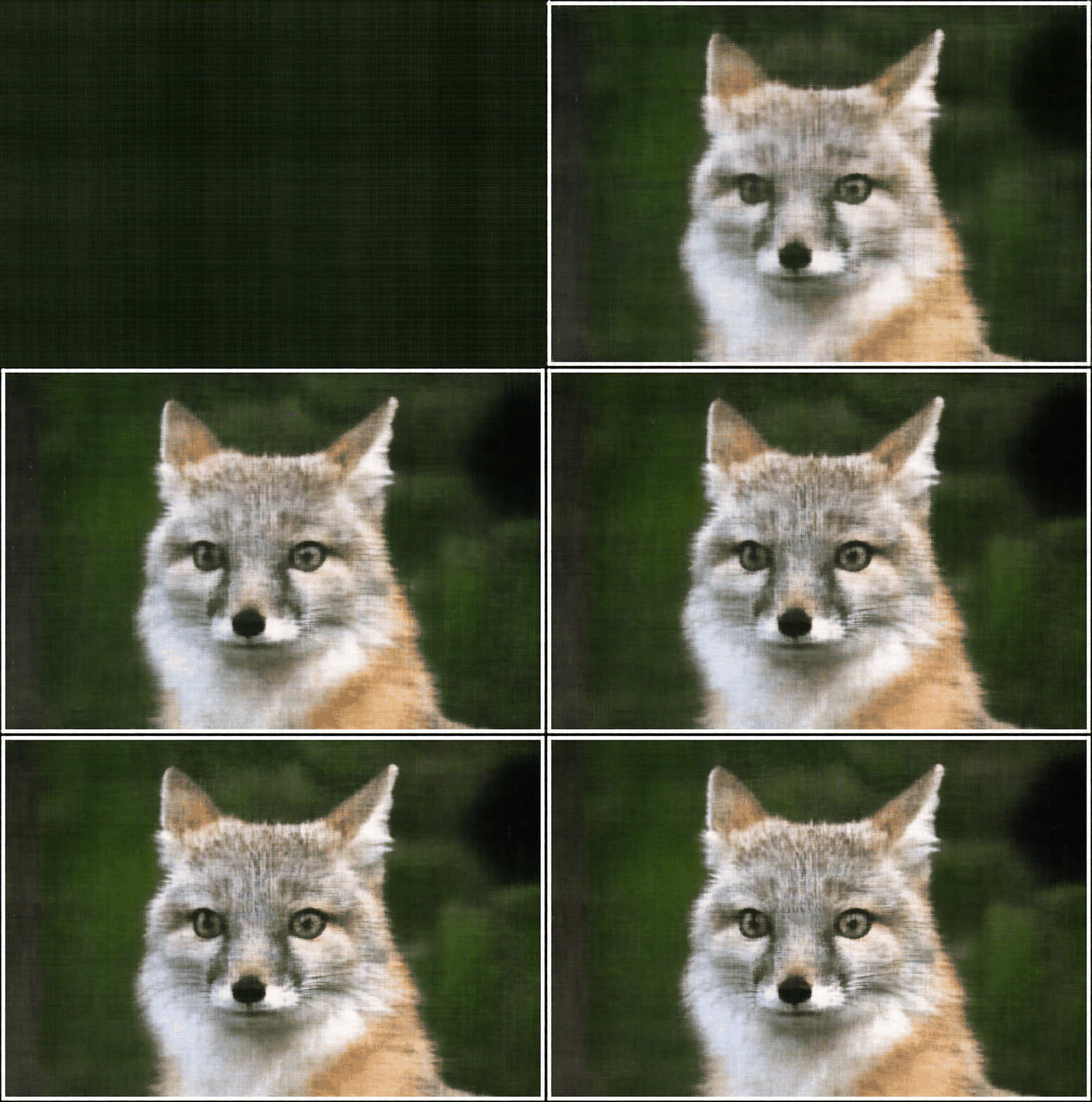
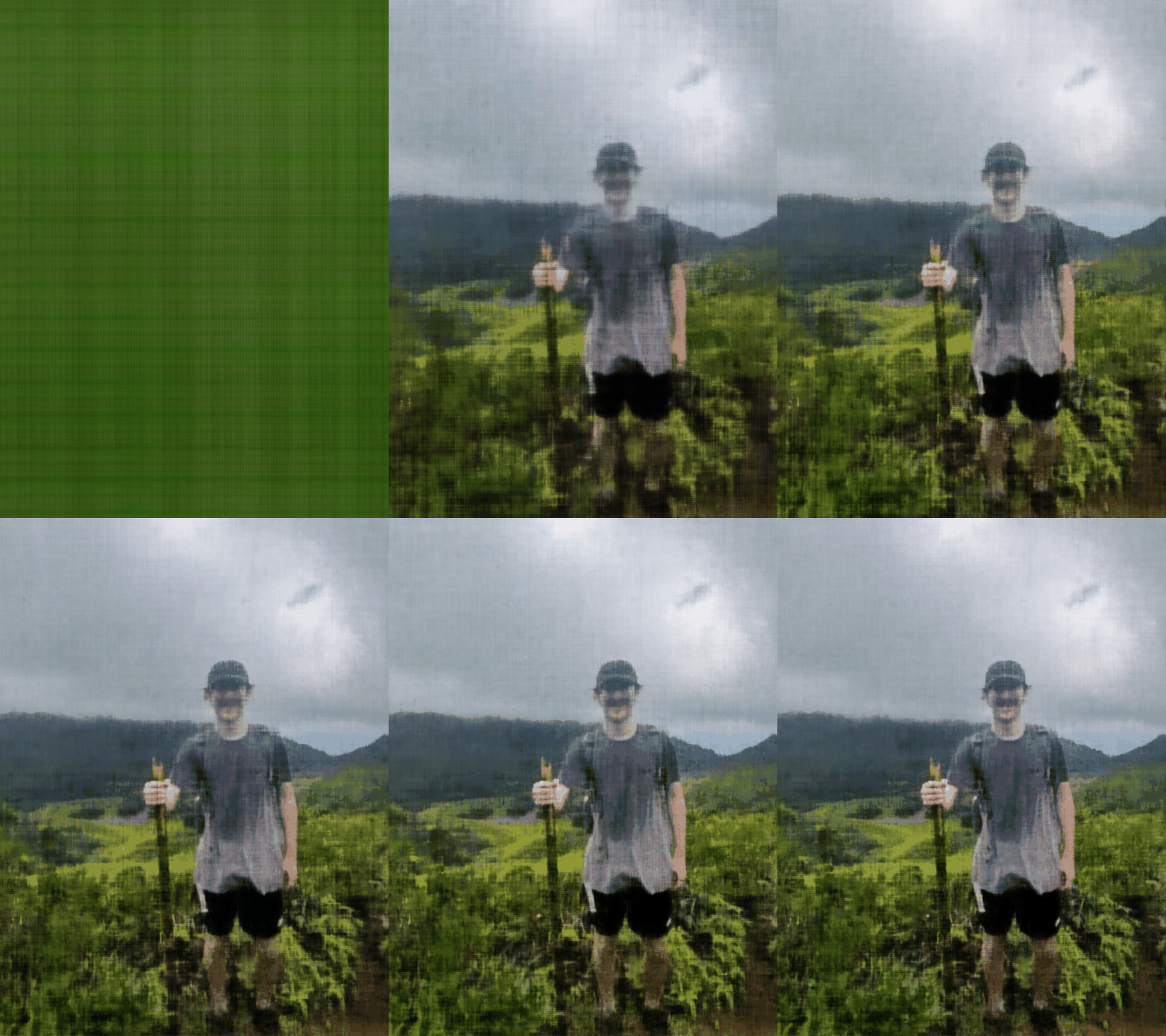
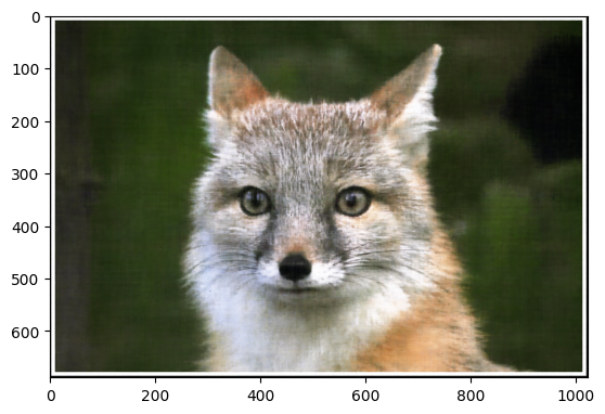
Next, we try a different set of hyperparameters and see how it affects the results. I tried a lower learning rate (5e-3) along with a higher max frequency (L=20) for the PE. This lead to slightly improved results on the Fox, as shown below. Notice the peak PSNR is higher than before.

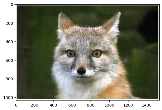
[Bells & Whistles] Interestingly, if we increase the resolution of our rendered images (say by some resolution factor $\alpha$), the quality of our image remains. I expected some artifacts to show up along the lines of out-of-distribution inputs, but the learned reconstruction was able to successfully interpolate on the unseen inputs.

Part 2: Fit a Neural Radiance Field from Multi-view Images
Now that we are familiar with using a neural field to represent a image, we proceed by using a neural radiance field to represent a 3D space, through inverse rendering from multi-view calibrated images. For this part we are going to use the Lego scene from the original NeRF paper, but with lower resolution images and preprocessed cameras.
Part 2.1: Create Rays from Cameras
First, we implement functions for (1) camera to world coordinate conversion, (2) pixel to camera
coordinate conversion, and (3) pixel to ray.
To implement (1), we write a function that performs the following:
$$
\begin{bmatrix}
x_c \\
y_c \\
z_c \\
1
\end{bmatrix}
=
\begin{bmatrix}
\mathbf{R}_{3 \times 3} & \mathbf{t} \\
\mathbf{0}_{1 \times 3} & 1
\end{bmatrix}
\begin{bmatrix}
x_w \\
y_w \\
z_w \\
1
\end{bmatrix}
$$
To implement (2), we write a function that performs the following:
$$ s
\begin{bmatrix}
u \\
v \\
1
\end{bmatrix}
=
\mathbf{K}
\begin{bmatrix}
x_c \\
y_c \\
1
\end{bmatrix}
$$
To implement (3), we define a ray as an origin $\mathbf{r}_o\in\mathbb{R}^3$ and
a direction $\mathbf{r}_d\in\mathbb{R}^3$. In order to know $\left[\mathbf{r}_o,
\mathbf{r}_d\right]$ for each $(u,v)$, we can perform the following:
$$\mathbf{r}_o=-\mathbf{R}_{3 \times 3}^{-1}\mathbf{t}$$
$$\mathbf{r}_d=\frac{\mathbf{X}_{\mathbf{w}}-\mathbf{r}_o}{
\|\mathbf{X}_{\mathbf{w}}-\mathbf{r}_o\|_2
}$$
Part 2.2: Sampling
Now, we use the three functions we implemented in the previous part to allow for (1)
sampling rays from images and (2) sampling points along rays.
In order to accomplish (1),
we flatten all pixels from all images and do a global sampling once to get N rays from all images.
To implement (2), we discritize each ray into samples that live in the 3D space. We do this
by uniformly sampling along the ray, but during training we introduce small perturbations to
avoid overfitting.
Part 2.3: Putting the Dataloading All Together
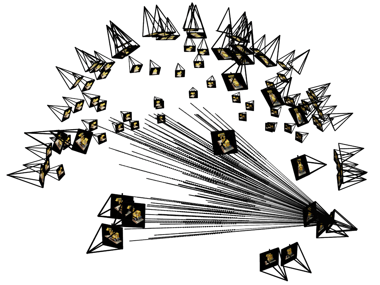
Next, we verify that our sampling is correct by writing a dataloader. We use viser to visualize the cameras, rays, and samples in 3D.
Part 2.4: Neural Radiance Field
Below is the architecture that we implement. Notice that this MLP is noticeably deeper than before. This is due to the fact that we are doing a more challenging task of optimizing a 3D representation rather than a 2D representation, so we need network with higher capacity.

Part 2.5: Volume Rendering
Next we implement the volume rendering equation. The core volume rendering equation is as follows:
$$C(\mathbf{r})=\int_{t_n}^{t_f}T(t)\sigma(\mathbf{r}(t))\mathbf{c}(\mathbf{r}(t))dt,$$
where $T(t)=\exp\left(-\int_{t_n}^{t}\sigma(\mathbf{r}(s))ds\right)$. The discrete (and tractable)
approximation, which we implement, is as follows:
$$\hat{C}(\mathbf{r})=\sum_{i=1}^NT_i(1-\exp(-\sigma_i\delta_i))\mathbf{c}_i,$$
where $T_i=\exp\left(\sum_{j=1}^{i-1}\sigma_j\delta_j\right)$, $\mathbf{c}_i$ is the color returned
by the network at sample location $i$, $T_i$ is the probability a ray not termininating before sample
location $i$, and $1-\exp(-\sigma_i\delta_i)$ is the probability of terminating at sample location $i$.
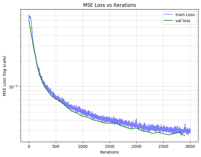
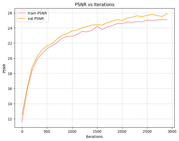
Finally, we are ready to train our model. We use L1=20, L2=10 for the $x$ and $r_d$ PE respectively,
an Adam optimizer with a learning rate of 5e-4, and a batchsize of 10k rays per iteration. This yields the
following loss and PSNR curves (training and validation):
The following showcases predicted images on the validation set as the model trains:


Finally, we can render novel views, as shown below with spherical renderings of the lego scene.
